Recognizing Individual Characters

[moonlitegram]

Hi All,

I've run into a little bit of a wall. When I try to perform a lookup, or a countif, excel treats a set of letter or numbers in the cell as one character. For example, SUG - I want to be able to single out the S in the cell, but excell will only recognize countifs and lookups for "SUG". I know FIND and SEARCH can do this, but I can't seem to get them to work for an entire column, only for one cell. Is there a function to search for specific characters down an entire column?

If it helps, this is what I'm trying to accomplish:

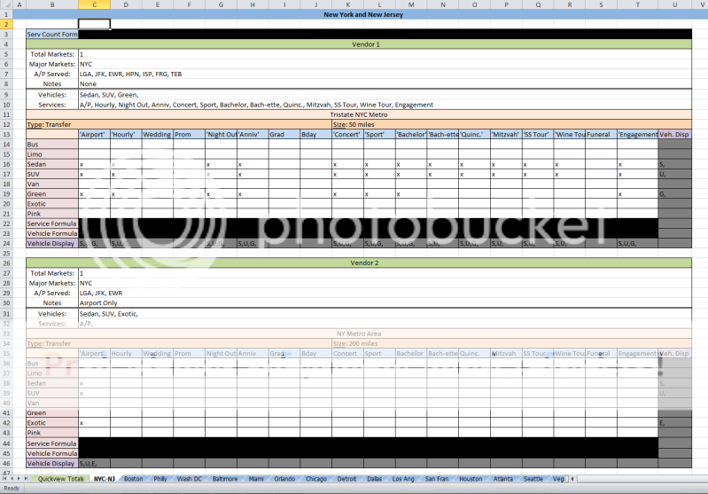
For a car service site I've created a sheet which contains multiple "profile" tables of vendor accounts and the vehicles and services they offer. The tables are simple, vehicles run down the rows and services go across colums. I've then nested some formulas so i can x off the vehicle boxes in each service and have it automate information.

One of the things it does is add a vehicle code (a letter) for each vehicle under each service. So if the vendor offers airport service with a Sedan, Van and an Green vehicle, S,U,G, is listed under that service. If they have a bus, and i click it on, it will read B, S, U, G and so forth.

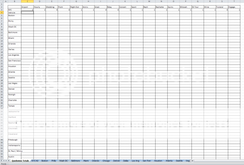
There are multiple profile tables on the sheet lined up directly underneath each other and eventually an admin will be able to continue to add the tables in for new vendors. I want excel to search down a colum, say the B column, and reproduced the results into a single cell so that I can reference that cell an seperate master sheet.

So if there are three vendors with airport service and their vehicle set ups look like this:
Vendor A - S, V, G
Vendor B - B, G, E
Vendor C - V, U, S,

I would want excel to search the column and display in one cell B, S, U, V, G, E.

Any help in this would be great appreciated! Since Excel automatically counts the letter combinations as a new character so far my only solution involves a formula with over 54 thousand IF functions - so that's not going to work lol

Thanks again!

 

[Scott Huish]

Since Excel automatically counts the letter combinations as a new character so far my only solution involves a formula with over 54 thousand IF functions - so that's not going to work lol

What are you talking about?

COUNTIF can take wildcards.

But you also say this:

I would want excel to search the column and display in one cell B, S, U, V, G, E.

Didn't you want a count?

Sheet1

<TABLE style="BACKGROUND-COLOR: #ffffff; PADDING-LEFT: 2pt; PADDING-RIGHT: 2pt; FONT-FAMILY: Calibri,Arial; FONT-SIZE: 11pt" border=1 cellSpacing=0 cellPadding=0><COLGROUP><COL style="WIDTH: 30px; FONT-WEIGHT: bold"><COL style="WIDTH: 173px"><COL style="WIDTH: 119px"><COL style="WIDTH: 183px"><COL style="WIDTH: 64px"><COL style="WIDTH: 64px"><COL style="WIDTH: 64px"></COLGROUP><TBODY><TR style="TEXT-ALIGN: center; BACKGROUND-COLOR: #cacaca; FONT-SIZE: 8pt; FONT-WEIGHT: bold"><TD> </TD><TD>A</TD><TD>B</TD><TD>C</TD><TD>D</TD><TD>E</TD><TD>F</TD></TR><TR style="HEIGHT: 18px"><TD style="TEXT-ALIGN: center; BACKGROUND-COLOR: #cacaca; FONT-SIZE: 8pt">1</TD><TD>Vendor A</TD><TD>S, V, G</TD><TD> </TD><TD>Count of:</TD><TD>B</TD><TD style="TEXT-ALIGN: right">1</TD></TR><TR style="HEIGHT: 18px"><TD style="TEXT-ALIGN: center; BACKGROUND-COLOR: #cacaca; FONT-SIZE: 8pt">2</TD><TD>Vendor B</TD><TD>B, G, E</TD><TD> </TD><TD>Count of:</TD><TD>S</TD><TD style="TEXT-ALIGN: right">2</TD></TR><TR style="HEIGHT: 18px"><TD style="TEXT-ALIGN: center; BACKGROUND-COLOR: #cacaca; FONT-SIZE: 8pt">3</TD><TD>Vendor C</TD><TD>V, U, S</TD><TD> </TD><TD>Count of:</TD><TD>U</TD><TD style="TEXT-ALIGN: right">1</TD></TR><TR style="HEIGHT: 18px"><TD style="TEXT-ALIGN: center; BACKGROUND-COLOR: #cacaca; FONT-SIZE: 8pt">4</TD><TD> </TD><TD> </TD><TD> </TD><TD>Count of:</TD><TD>V</TD><TD style="TEXT-ALIGN: right">2</TD></TR><TR style="HEIGHT: 18px"><TD style="TEXT-ALIGN: center; BACKGROUND-COLOR: #cacaca; FONT-SIZE: 8pt">5</TD><TD> </TD><TD> </TD><TD> </TD><TD>Count of:</TD><TD>G</TD><TD style="TEXT-ALIGN: right">2</TD></TR><TR style="HEIGHT: 18px"><TD style="TEXT-ALIGN: center; BACKGROUND-COLOR: #cacaca; FONT-SIZE: 8pt">6</TD><TD> </TD><TD> </TD><TD> </TD><TD>Count of:</TD><TD>E</TD><TD style="TEXT-ALIGN: right">1</TD></TR></TBODY></TABLE>
<TABLE style="BORDER-BOTTOM-STYLE: groove; BORDER-BOTTOM-COLOR: #00ff00; BACKGROUND-COLOR: #fffcf9; BORDER-TOP-COLOR: #00ff00; BORDER-LEFT-STYLE: groove; FONT-FAMILY: Arial; BORDER-TOP-STYLE: groove; COLOR: #000000; BORDER-RIGHT-COLOR: #00ff00; BORDER-RIGHT-STYLE: groove; FONT-SIZE: 10pt; BORDER-LEFT-COLOR: #00ff00"><TBODY><TR><TD>Spreadsheet Formulas</TD></TR><TR><TD><TABLE style="FONT-FAMILY: Arial; FONT-SIZE: 9pt" border=1 cellSpacing=0 cellPadding=2><TBODY><TR style="BACKGROUND-COLOR: #cacaca; FONT-SIZE: 10pt"><TD>Cell</TD><TD>Formula</TD></TR><TR><TD>F1</TD><TD>=COUNTIF(B:B,"*"&E1&"*")</TD></TR><TR><TD>F2</TD><TD>=COUNTIF(B:B,"*"&E2&"*")</TD></TR><TR><TD>F3</TD><TD>=COUNTIF(B:B,"*"&E3&"*")</TD></TR><TR><TD>F4</TD><TD>=COUNTIF(B:B,"*"&E4&"*")</TD></TR><TR><TD>F5</TD><TD>=COUNTIF(B:B,"*"&E5&"*")</TD></TR><TR><TD>F6</TD><TD>=COUNTIF(B:B,"*"&E6&"*")</TD></TR></TBODY></TABLE></TD></TR></TBODY></TABLE>

Excel tables to the web >> http://www.excel-jeanie-html.de/index.php?f=1" target="_blank"> Excel Jeanie HTML 4

 

[moonlitegram]

Thanks for the response hotpepper. Perhaps it would be more clear if I posted images

You can see the two vendor "profiles" in the pic above. In column C I have a cell highlighted up top that I'd like to return the vehicle codes that appear down that C column. So in the example of this image the final result would be S, U, G, E because Vendor 1 has SUG and Vendor 2 has SUE

It's necessary to combine all the vendors vehicle types in this column because I'm going to reference it on a master page for a quick overveiw of services and vehicles in each market. See image below:

The plan was to nest a formula for each service column on the original image so I can reference it under the vehicle category for each market in the second image. Make sense?

 

[Marcelo Branco]

Maybe this UDF (User Defined Function)

Paste the code below in a Standard Module
Alt+F11 to open the VBEditor
Insert > Module
Paste in the right panel

Function aTest(ParamArray r() As Variant)
    Dim i As Long, s As Variant, rCell As Variant
    Dim strResult As String
 
    For Each rCell In r
        If TypeOf rCell Is Range Then
            s = Split(Application.Substitute(rCell, " ", ""), ",")
            For i = LBound(s) To UBound(s)
                If InStr(1, strResult, s(i)) = 0 Then strResult = strResult & s(i) & ", "
            Next i
        End If
    Next rCell
 
    aTest = Left(strResult, Len(strResult) - 2)
 
End Function

Usage

C2
=aTest(C24,C46)

M.

 

[moonlitegram]

Thanks for help Marcelo. I appreciate it.

Although its not exactly what I need. I need a function where I can give it an entire range of cells in the C column (as an admin will be adding more of those profile cards in the future) rather than specific cells.

The real issue comes from excel treating SUG as "SUG" and not "S" "U" and "G". If I can get excel to treat them as individual letters I could easily create a formula using IF and CountIF or Lookup functions.

The SEARCH function allows me to search for individual letters but I can't get it to search an entire column of cells for the text, only one cell at a time. If I could get it to search the entire column Id have my problem solved as well.

Any ideas?
Thanks

 

[moonlitegram]

I was able to figure the issue out. I'm updating this post for anyone seeking similar future advice. The solution involves using the IF(ISNUMBER(SEARCH function as an array formula.

Excel - Search Function for multiple cells. The Fucntion I used was:

IF(--ISNUMBER(SEARCH("criteria",range)))>0,"True Value","False Value")
Enter the forumula using Shift+Ctrl+Enter to make it an array formula.