Search and result

[jigarecity]

Dear All,

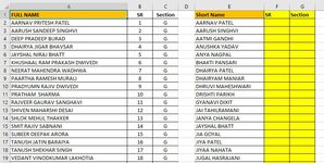
kindly find attached photo of data ..

in A column FULL NAME LIST available with SR & Section
in E column short Name list available

Now i have to search short name (F2 Cell) from A column and given result in G & H for SR & Section in yellow area ..

hope you understand my problem.. if you have any query please feel free to revert.

Thanks in Advance
jigarecity

 

[jtakw]

Hi,

Please post samples using XL2BB so that we don't have to manually recreate your data for testing, see my signature for where and how.
Is this what you need?

Book3.xlsx
	A	B	C	D	E	F
1		SR	Section		SR	Section
2	john jack doe	1	A	jane abc	2	B
3	jane jill abc	2	B	jack jill	Not Listed	Not Listed
4	joe doe jack	3	C	john doe	1	A
5
6
7
8
9
10
Sheet908

Cell Formulas
Range	Formula
E2:F4	E2	=IFERROR(LOOKUP(2,1/SEARCH(LEFT($D2,FIND(" ",$D2))&"*"&MID($D2,FIND(" ",$D2),99),$A$2:$A$10),B$2:B$10),"Not Listed")

 

[Fluff]

Welcome to the MrExcel Message Board!

Cross-posting (posting the same question in more than one forum) is not against our rules, but the method of doing so is covered by #13 of the Forum Rules.

Be sure to follow & read the link at the end of the rule too!

Cross posted at: Search and result
If you have posted the question at more places, please provide links to those as well.

If you do cross-post in the future and also provide links, then there shouldn’t be a problem.

 

[jigarecity]

Hi,

Please post samples using XL2BB so that we don't have to manually recreate your data for testing, see my signature for where and how.
Is this what you need?

Book3.xlsx
	A	B	C	D	E	F
1		SR	Section		SR	Section
2	john jack doe	1	A	jane abc	2	B
3	jane jill abc	2	B	jack jill	Not Listed	Not Listed
4	joe doe jack	3	C	john doe	1	A
5
6
7
8
9
10
Sheet908

Cell Formulas
Range	Formula
E2:F4	E2	=IFERROR(LOOKUP(2,1/SEARCH(LEFT($D2,FIND(" ",$D2))&"*"&MID($D2,FIND(" ",$D2),99),$A$2:$A$10),B$2:B$10),"Not Listed")

Thank you very much
it's work perfectly
5*

 

[kvsrinivasamurthy]

In F2 then copied across and Down till required.

=IFERROR(INDEX(B$3:B$19,AGGREGATE(15,6,ROW($A$3:$A$19)/((ISNUMBER(SEARCH(LEFT($E2,FIND(" ",$E2)-1),$A$3:$A$19))+ISNUMBER(SEARCH(RIGHT($E2,LEN($E2)-FIND(" ",$E2)),$A$3:$A$19)))=2),1)-ROW($A$2)),"")

In range $A$3:$A$19 19 can be changed as required.

 

[jtakw]

Thank you very much
it's work perfectly
5*

You're welcome, thanks for the feedback.

Don't forget to mark the post that solved your question as solution. Thank you.