Sequence Values In order but need to be Unique

Riddlemethis

New Member
Joined
Apr 20, 2021
Messages
14
Office Version
  1. 2013
Platform
  1. Windows
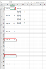
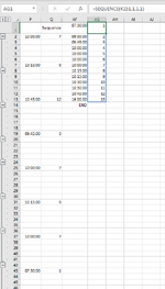
Data dump fills out cells. In Column P the data will give the start time of certain shifts.
Column AG will have a sequence of numbers 1 to whatever the total number of start times there is that day.
Column AF fills out after macro is run to copy and paste the start times.
Column Q returns the Sequence number via vlookup.

So problem being i would need each start time to have it's own unique number even though there may be more that one say 09:00:00 start time... As you can see
Is their a method to have the sequence or vlookup return a unique value if there is a duplicate value dropped into AF? It doesn't matter what it returns as long as the value is higher than a start time earlier an lower than a start time later.
 

Attachments

  • Start Time Sequence.png
    Start Time Sequence.png
    25.8 KB · Views: 9
  • Start Time Sequence 2.png
    Start Time Sequence 2.png
    23.3 KB · Views: 10
Last edited:

Excel Facts

How can you automate Excel?
Press Alt+F11 from Windows Excel to open the Visual Basic for Applications (VBA) editor.
Is this what you mean?

BTW, I suggest that you investigate XL2BB for providing sample data to make it easier for helpers by not having to manually type out sample data to test with.

22 11 27.xlsm
PQAFAG
107:30:001
210:00:00409:00:002
3 09:45:003
410:15:00810:00:004
5 10:00:005
610:45:00 10:00:006
7 10:00:007
809:45:00310:15:008
9 10:15:009
1010:00:005
11 
1210:15:009
13 
1410:00:006
Sequence
Cell Formulas
RangeFormula
Q2:Q14Q2=IFERROR(AGGREGATE(15,6,$AG$1:$AG$150/($AF$1:$AF$150=P2),COUNTIF($P$2:$P2,$P2)),"")
 
Upvote 0
My Bad, I knew XL2BB existed and was lazy on this one..

Your solution is almost perfect and appreciated. is it possible though for the first value in your formula to be '1' and not blank? as in cell Q55

DRB Test.xlsm
PQAFAG
1Sequence09:00:001
210:00:00409:00:002
3 009:30:003
4 010:00:004
5 010:30:005
6 010:30:006
7 011:00:007
809:30:00311:30:008
9 011:30:009
10 013:00:0010
11 014:00:0011
12 0END
13 0
1410:30:005
15 0
16 0
17 0
18 0
19 0
2009:00:002
21 0
22 0
23 0
24 0
25 0
2611:30:008
27 0
28 0
29 0
30 0
31 0
3214:00:0011
33 0
34 0
35 0
36 0
3711:30:009
38 0
39 0
40 0
41 0
42 0
4311:00:007
44 0
45 0
46 0
47 0
48 0
4910:30:006
50 0
51 0
52 0
53 0
54 0
5509:00:00 
56 0
57 0
58 0
59 0
60 0
6113:00:0010
62 0
63 0
64 0
65 0
66END0
67 0
68 0
69 0
Data
Cell Formulas
RangeFormula
AG1:AG11AG1=SEQUENCE(K151,1,1,1)
P2:P69P2=IFS(K2=1,(RIGHT(D3,8)),L2=1,(RIGHT(D3,8)),M2=1,(RIGHT(D3,8)),N2=1,"END",TRUE,"")
Q2:Q69Q2=IFERROR(AGGREGATE(15,6,$AG$2:$AG$150/($AF$2:$AF$150=P2),COUNTIF($P$2:$P2,$P2)),"")
Dynamic array formulas.
 
Upvote 0
There are, or could be, a few issues.
  1. Your formulas in column P refer to a different row on the left of the sheet. For example, the P2 formula refers to K2:N2 but then D3. Is that correct?
  2. The formulas in column P are returning a text time but the times in column AF appear to be actual times (that is, numbers)
  3. I had made a mistake with my column Q formula (corrected since but looks like you had seen & used the original). The table in columns AF:AG starts in row 1, not row 2
So, try this revised formula in P2. It should address points 2 and 3 above.

Excel Formula:
=IFERROR(AGGREGATE(15,6,$AG$1:$AG$150/($AF$1:$AF$150=P2+0),COUNTIF($P$2:$P2,$P2)),"")
 
Upvote 0
Solution
getting all "" ( Blanks ) now. Tried formatting all 3 columns as text time and general and getting "" as the result either way. In regards to your points 1 & 2 you correct in both. Opening this up as much as i can as i appreciate your efferts altough now I think the outcome will be towards my inventable daftness in formatting data correctly??

SequenceTURun Drop 1Drop 2Drop 3Drop 4Drop 5Drop 6Drop 7Drop 8Start TriggerGap CountShift Type09:00:001
110:00:0015DoubleShift09:00:002
09:30:003
45686NI660NI66010:00:004
45707NI415,NI412,NI989,NI416NI415NI412NI989NI41610:30:005
45697NI989,NI412NI989NI41210:30:006
45681NI407,NI563NI407NI56311:00:007
109:30:0015DoubleShift11:30:008
11:30:009
45710NI980,NI422NI980NI42213:00:0010
45678NI996,NI420NI996NI42014:00:0011
45665NI401,NI661NI401NI661END
45692NI980,NI982NI980NI982
110:30:0015DoubleShift
45700NI411,NI993NI411NI993
45689NI402,NI678NI402NI678
45664NI989,NI400NI989NI400
45711NI403,NI422NI403NI422
109:00:0015DoubleShift
45704NI406,NI414,NI407NI406NI414NI407
45679NI566,NI424NI566NI424
45682NI564,NI998NI564NI998
45690NI980NI980
111:30:0015DoubleShift
45708NI413,NI401,NI424,NI566NI413NI401NI424NI566
45673NI414,NI564NI414NI564
45680NI411,NI528NI411NI528
45667NI403,NI418NI403NI418
114:00:00143x3
45668NI406NI406
45691NI981NI981
45685NI650NI650
111:30:0015DoubleShift
45666NI402,NI418NI402NI418
45688NI998,NI413NI998NI413
45676NI982,NI417NI982NI417
45669NI407NI407
111:00:0015DoubleShift
45702NI997NI997
45709NI420,NI998,NI400,NI661NI420NI998NI400NI661
45670NI981,NI408NI981NI408
45699NI982,NI991NI982NI991
110:30:0015DoubleShift
45672NI416,NI412NI416NI412
45705NI411,NI996,NI986,NI564NI411NI996NI986NI564
45698NI990,NI987NI990NI987
45696NI988NI988
109:00:0015DoubleShift
45674NI567,NI996NI567NI996
45706NI660,NI650,NI983,NI678NI660NI650NI983NI678
45684NI567,NI997NI567NI997
45693NI983NI983
113:00:00143x3
45694NI986NI986
45687NI661NI661
45695NI987NI987
1END1?END
 
Upvote 0
Tried formatting all 3 columns as ..
Changing the format of a column does not change the underlying values in the cells. If they are text then they stay as text etc. Formatting only (possibly) changes the appearance.

Can you post that XL2BB again using Mini Sheet not Table Only after you have first hidden the irrelevant columns? Can you ensure we see columns D, P, Q (with my formula inserted in that column), AF & AG. About 30 rows should be plenty.
 
Upvote 0
DRB Test.xlsm
DPQAFAG
1StartSequence09:00:001
210:00:00 09:00:002
327.11 10:00:00  09:30:003
427.11 10:00:00  10:00:004
527.11 14:23:36  10:30:005
627.11 20:46:54  10:30:006
728.11 01:43:30  11:00:007
809:30:00 11:30:008
927.11 09:30:00  11:30:009
1027.11 09:30:00  13:00:0010
1127.11 17:01:30  14:00:0011
1227.11 21:03:54  END
1328.11 00:56:48  
1410:30:00 
1527.11 10:30:00  
1627.11 10:30:00  
1727.11 15:31:48  
1827.11 20:33:42  
1928.11 01:11:18  
2009:00:00 
2127.11 09:00:00  
2227.11 09:00:00  
2327.11 16:19:30  
2427.11 20:00:42  
2528.11 00:22:42  
2611:30:00 
2727.11 11:30:00  
2827.11 11:30:00  
2927.11 15:59:30  
3027.11 22:48:00  
3128.11 03:35:36  
3214:00:00 
3327.11 14:00:00  
3427.11 14:00:00  
3527.11 17:50:58  
3627.11 22:26:04  
3711:30:00 
3827.11 11:30:00  
3927.11 11:30:00  
4027.11 16:27:06  
4127.11 21:31:30  
4228.11 02:07:54  
4311:00:00 
4427.11 11:00:00  
4527.11 11:00:00  
4627.11 15:14:12  
4727.11 20:28:12  
4828.11 00:57:36  
4910:30:00 
Data
Cell Formulas
RangeFormula
AG1:AG11AG1=SEQUENCE(K151,1,1,1)
P2:P49P2=IFS(K2=1,(RIGHT(D3,8)),L2=1,(RIGHT(D3,8)),M2=1,(RIGHT(D3,8)),N2=1,"END",TRUE,"")
Q2:Q49Q2=IFERROR(AGGREGATE(15,6,$AG$1:$AG$150/($AF$1:$AF$150=P2+0),COUNTIF($P$2:$P2,$P2)),"")
Dynamic array formulas.
 
Upvote 0
You're welcome. Glad you got it working. Thanks for the follow-up. :)
 
Upvote 0

Forum statistics

Threads
1,214,979
Messages
6,122,561
Members
449,089
Latest member
Motoracer88

We've detected that you are using an adblocker.

We have a great community of people providing Excel help here, but the hosting costs are enormous. You can help keep this site running by allowing ads on MrExcel.com.
Allow Ads at MrExcel

Which adblocker are you using?

Disable AdBlock

Follow these easy steps to disable AdBlock

1)Click on the icon in the browser’s toolbar.
2)Click on the icon in the browser’s toolbar.
2)Click on the "Pause on this site" option.
Go back

Disable AdBlock Plus

Follow these easy steps to disable AdBlock Plus

1)Click on the icon in the browser’s toolbar.
2)Click on the toggle to disable it for "mrexcel.com".
Go back

Disable uBlock Origin

Follow these easy steps to disable uBlock Origin

1)Click on the icon in the browser’s toolbar.
2)Click on the "Power" button.
3)Click on the "Refresh" button.
Go back

Disable uBlock

Follow these easy steps to disable uBlock

1)Click on the icon in the browser’s toolbar.
2)Click on the "Power" button.
3)Click on the "Refresh" button.
Go back
Back
Top