Simple Tweak in VBA required while copying data from one sheet to another

[Jyotirmaya]

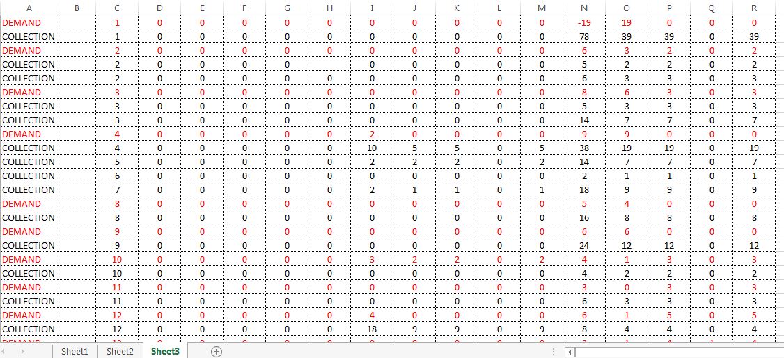
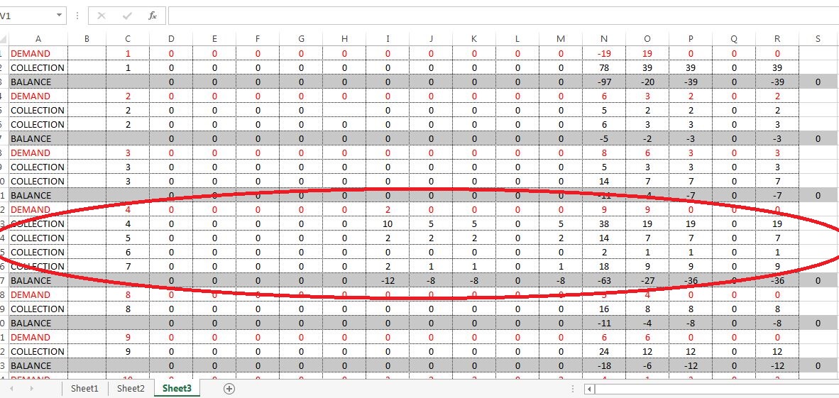
I want to copy my data of "Sheet 1" and "sheet 2" to "sheet 3"

I have the following code

Sub sbCopyRangeToAnotherSheet()
Sheets("Sheet1").Range("A1:P100").Copy
Sheets("Sheet3").Activate
ActiveSheet.Paste
Application.CutCopyMode = False
End Sub

1. Now I want the copied data of sheet1 in sheet3 should be of BLUE color
2. After copying Shee1's data in sheet3, Sheet2's data will copy below to the Sheet1's data & of which Green color.
3. After copying both data Column C will be sorted from smallest to largest.

 

[ZVI]

You may start with such a code

Sub Test1()
 
  Dim Sh1 As Worksheet, Sh3 As Worksheet, Sh2 As Worksheet
 
  ' This provides IntelliSense
  Set Sh1 = Sheets("Sheet1")
  Set Sh2 = Sheets("Sheet2")
  Set Sh3 = Sheets("Sheet3")
   
  Sh3.UsedRange.Clear
 
  Sh1.Range("A1:P100").Copy Sh3.Cells(1, 1)
  Sh3.Range("A1:P100").Font.Color = vbBlue
 
  Sh2.Range("A1:P100").Copy Sh3.Cells(101, 1)
  Sh3.Range("A101:P201").Font.Color = vbGreen
 
  Sh3.UsedRange.Sort Key1:=Sh3.Cells(1, 3), Order1:=xlAscending, Header:=xlGuess
 
End Sub

 

[ZVI]

Or use this in case copying of all data from Sh1 & Sh2 into Sh3 is required

Sub Test2()
 
  Dim Sh1 As Worksheet, Sh3 As Worksheet, Sh2 As Worksheet
  Dim n1 As Long, n2 As Long
 
  ' This provides IntelliSense
  Set Sh1 = Sheets("Sheet1")
  Set Sh2 = Sheets("Sheet2")
  Set Sh3 = Sheets("Sheet3")
 
  ' Data rows count in Sheet1 and Sheet2 accordingly
  n1 = Sh1.UsedRange.Rows.Count
  n2 = Sh2.UsedRange.Rows.Count
 
  ' Clear Sh3
  Sh3.UsedRange.Clear
 
  ' Copy Sh1 to Sh3
  Sh1.UsedRange.Copy Sh3.Cells(1, 1)
  Sh3.UsedRange.Font.Color = vbBlue  ' or may be Sh3.UsedRange.Interior.Color = vbBlue
 
  ' Copy Sh2 to Sh3
  Sh2.UsedRange.Copy Sh3.Cells(n1 + 1, 1)
  Sh3.UsedRange.Rows(n1 + 1 & ":" & n1 + n2 + 1).Font.Color = vbGreen
 
  ' Sort column C of Sh3
  Sh3.UsedRange.Sort Key1:=Sh3.Cells(1, 3), Order1:=xlAscending, Header:=xlGuess
 
End Sub

 

[ZVI]

Typo: n1 + n2 + 1
Please correct it to: n1 + n2

 

[Jyotirmaya]

You may start with such a code

Sub Test1()
 
  Dim Sh1 As Worksheet, Sh3 As Worksheet, Sh2 As Worksheet
 
  ' This provides IntelliSense
  Set Sh1 = Sheets("Sheet1")
  Set Sh2 = Sheets("Sheet2")
  Set Sh3 = Sheets("Sheet3")
   
  Sh3.UsedRange.Clear
 
  Sh1.Range("A1:P100").Copy Sh3.Cells(1, 1)
  Sh3.Range("A1:P100").Font.Color = vbBlue
 
  Sh2.Range("A1:P100").Copy Sh3.Cells(101, 1)
  Sh3.Range("A101:P201").Font.Color = vbGreen
 
  Sh3.UsedRange.Sort Key1:=Sh3.Cells(1, 3), Order1:=xlAscending, Header:=xlGuess
 
End Sub

THANK YOU SO MUCH, YOU SAVED A LOT OF TIME, Its working,
1. what should be change in the code if I want to paste the data after C4 in Sheet3
2. What should be the change in code if I want to sort column 5

 

[ZVI]

THANK YOU SO MUCH, YOU SAVED A LOT OF TIME, Its working,
1. what should be change in the code if I want to paste the data after C4 in Sheet3
2. What should be the change in code if I want to sort column 5

Glad it helped!

Some explanations:

1. For example, in this line Sh1.Range("A1:P100").Copy Sh3.Cells(1, 1)
the destination cell is Sh3.Cells(1, 1) where Cells(row, column) is referred to A1 because its row=1 and column=1.
For C4 it would be Sh3.Cells(4, 3) where 4 is the row and 3 is column number of С4. Or use Sh3.Range("C4")
Provide also changing of other ranges referencing/offsetting in the code.
Please read more details about Cells property and Copy method for Range object in VBA help.

2. In this line of code Sh3.UsedRange.Sort Key1:=Sh3.Cells(1, 3), Order1:=xlAscending, Header:=xlGuess
that part Key1:=Sh3.Cells(1, 3) is reffered to C1 cell because its row=1 and column=3, change it as required,
for example to Key1:=Sh3.Cells(5, 3) or to Key1:=Sh3.Range("C5")

 

[Jyotirmaya]

Glad it helped!

Some explanations:

1. For example, in this line Sh1.Range("A1:P100").Copy Sh3.Cells(1, 1)
the destination cell is Sh3.Cells(1, 1) where Cells(row, column) is referred to A1 because its row=1 and column=1.
For C4 it would be Sh3.Cells(4, 3) where 4 is the row and 3 is column number of С4. Or use Sh3.Range("C4")
Provide also changing of other ranges referencing/offsetting in the code.
Please read more details about Cells property and Copy method for Range object in VBA help.

2. In this line of code Sh3.UsedRange.Sort Key1:=Sh3.Cells(1, 3), Order1:=xlAscending, Header:=xlGuess
that part Key1:=Sh3.Cells(1, 3) is reffered to C1 cell because its row=1 and column=3, change it as required,
for example to Key1:=Sh3.Cells(5, 3) or to Key1:=Sh3.Range("C5")

Amazing, I got that, but I have little more problem. After This macro I am using the below code

Sub try()
 Dim c As Range
 Dim lRow As Long
 lRow = 1
 Dim lRowLast As Long
 Dim lRowDiff As Long
 Dim lRowPortion As Long
 lRowPortion = 1
 Dim bFoundCollection As Boolean
 With ActiveSheet
  lRowLast = .Cells(.Rows.Count, 1).End(xlUp).Row
  Do
   Set c = .Range("A" & lRow)
   If c.Value Like "*COLLECTION*" Then
    bFoundCollection = True
   ElseIf bFoundCollection Then
    bFoundCollection = False
    If c.Value <> "BALANCE" Then
     c.EntireRow.Insert
     lRowLast = lRowLast + 1
     Set c = c.Offset(-1, 0)
     c.Value = "BALANCE"
    End If
    If c.Value = "BALANCE" Then
     .Range(c, c.Offset(0, 18)).Font.Color = RGB(0, 0, 0)
     .Range(c, c.Offset(0, 18)).Interior.Color = RGB(200, 200, 200)
     lRowDiff = c.Row - lRowPortion
     .Range(c.Offset(0, 3), c.Offset(0, 18)).FormulaR1C1 = _
      "=SUMIF(R[-" & lRowDiff & "]C1:RC1, ""*DEMAND*"", R[-" & lRowDiff & "]C:RC)" & _
      "-SUMIF(R[-" & lRowDiff & "]C1:RC1, ""*COLLECTION*"", R[-" & lRowDiff & "]C:RC)"
     lRowPortion = c.Row + 1
    End If
   End If
   lRow = lRow + 1
  Loop While lRow <= lRowLast + 1
 End With
End Sub

I use this code to Get the BALANCE, where BALANCE = DEMAND-COLLECTION
Column 3 defines the USER ID, and DEMAND means arrears due and Collection means amount collected from that User.
But the problem is when an user is not having any due but has paid certain amount. I am getting the below error, kindly check the image.
Image 1 - After the above code, After getting Balance

Image2 - Errors in the Sheet marked

From the image its concluded that there are no dues in USER ID 5 6 7 but still Collection has been done in favour of that USER ID. For such kind of problems I want to Move those Collection rows to the below of the sheet having Color Yellow, so that I can identify such users and can fix the error.

 

[ZVI]

Example of the code modification, where data is copied from Sh1 & Sh3 to Sh3 into cell C5 and to the cells below, then sorted by key of C5.

Sub Test1a()
 
  Dim Sh1 As Worksheet, Sh3 As Worksheet, Sh2 As Worksheet
 
  ' This provides IntelliSense
  Set Sh1 = Sheets("Sheet1")
  Set Sh2 = Sheets("Sheet2")
  Set Sh3 = Sheets("Sheet3")
   
  Sh3.UsedRange.Clear
 
  Sh1.Range("A1:P100").Copy Sh3.Range("C5")
  Sh3.Range("C5:R104").Font.Color = vbBlue
 
  Sh2.Range("A1:P100").Copy Sh3.Range("C105")
  Sh3.Range("C105:R204").Font.Color = vbGreen
 
  Sh3.Range("C5:R204").Sort Key1:=Sh3.Range("C5"), Order1:=xlAscending, Header:=xlGuess
 
End Sub

P.S. It's to my previous post

 

[ZVI]

From the image its concluded that there are no dues in USER ID 5 6 7 but still Collection has been done in favour of that USER ID. For such kind of problems I want to Move those Collection rows to the below of the sheet having Color Yellow, so that I can identify such users and can fix the error.

I see you are very comfortable with VBA and it's good!

Before running your Sub Try() you may isolate incorrect rows (may be to another sheet) as follows:

1. Apply such a formula to B2 and the cells below: =AND(C2<>C1,A2<>"DEMAND") like this:
Range("B2:B" & Cells(Rows.Count, 1).End(xlUp).Row).Formula = "=AND(C2<>C1,A2<>""DEMAND"")"

2. Filter column B by TRUE value in incorrect rows, color visible rows and then cut & paste it to another place

3. Clear column B. You may use any empty column instead of B

 

[ZVI]

2. Filter column B by TRUE value in incorrect rows, color visible rows and then cut & paste it to another place

To move incorrect rows to the bottom lines instead of filtering just sort column B.