This one is just out of interest
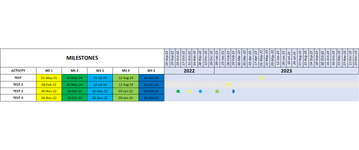
A colleague has sent over a spreadsheet which generates timelines based on dates contained in cols B - F
It used a series of dates at the top in row 2 from col g which are set up in 14 day intervals and then the rows below contain the formula below in order to populate the cells with specific characters depending on the dates in Cols B-F
Im sure there must be a simplified formula which will perform the same output
=IF(IFERROR(OR(I$2-$B6=-13,I$2-$B6=-12,I$2-$B6=-11,I$2-$B6=-10,I$2-$B6=-9,I$2-$B6=-8,I$2-$B6=-7,I$2-$B6=-6,I$2-$B6=-5,I$2-$B6=-4,I$2-$B6=-3,I$2-$B6=-2,I$2-$B6=-1,I$2-$B6=0),""),CHAR(186),IF(IFERROR(OR(I$2-$C6=-13,I$2-$C6=-12,I$2-$C6=-11,I$2-$C6=-10,I$2-$C6=-9,I$2-$C6=-8,I$2-$C6=-7,I$2-$C6=-6,I$2-$C6=-5,I$2-$C6=-4,I$2-$C6=-3,I$2-$C6=-2,I$2-$C6=-1,I$2-$C6=0),""),CHAR(190),IF(IFERROR(OR(I$2-$D6=-13,I$2-$D6=-12,I$2-$D6=-11,I$2-$D6=-10,I$2-$D6=-9,I$2-$D6=-8,I$2-$D6=-7,I$2-$D6=-6,I$2-$D6=-5,I$2-$D6=-4,I$2-$D6=-3,I$2-$D6=-2,I$2-$D6=-1,I$2-$D6=0),""),CHAR(191),IF(IFERROR(OR(I$2-$E6=-13,I$2-$E6=-12,I$2-$E6=-11,I$2-$E6=-10,I$2-$E6=-9,I$2-$E6=-8,I$2-$E6=-7,I$2-$E6=-6,I$2-$E6=-5,I$2-$E6=-4,I$2-$E6=-3,I$2-$E6=-2,I$2-$E6=-1,I$2-$E6=0),""),CHAR(192),IF(IFERROR(OR(I$2-$F6=-13,I$2-$F6=-12,I$2-$F6=-11,I$2-$F6=-10,I$2-$F6=-9,I$2-$F6=-8,I$2-$F6=-7,I$2-$F6=-6,I$2-$F6=-5,I$2-$F6=-4,I$2-$F6=-3,I$2-$F6=-2,I$2-$F6=-1,I$2-$F6=0),""),CHAR(187),"")))))
any ideas?