An alternative way to investigate this is to create a large table that covers the entire solution space and then use some visualization method to examine the results. In this case, I did this in two steps, but it could be streamlined somewhat. I first built a table describing the potential solution space. The body of the table is on sheet Data1 located at Data1!M13:HE213. From top to bottom, the rows represent seller 1 (S1) additional incentive products ranging from 0 (top) to 100,000 (bottom) in increments of 500. From left to right, the columns represent the sum of additional incentive products for both sellers (S1 + S2), ranging from 100,000 (left "M" column) to 0 (right, "HE" column), in decrements of 500. The body of the Data1 table then shows the number of additional incentive products for seller 2 (S2) that correspond to the column (total sum) given the S1 value of that row.
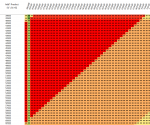
Then on another sheet called "HeatMap1", the S1 and S2 values in the "Data1" table are used to compute the sum of bonuses that would be awarded to each seller, and this calculation is done using the formula described previously (used twice...first to generate the bonus for seller 1 and again to generate the bonus for seller 2). Then conditional formatting was applied using 3-color formatting based on cell value, with the low global value assigned green, 40th percentile assigned yellow, and the high global value (170) assigned red. Then row and column sizes were shrunk to better visualize the entire space, producing this result:
If you look closely, you'll see a narrow vertical red bar about halfway down the left side, and to its right is a nearly complete red right triangle. Those areas correspond to optimal solutions; and zooming in on those areas looks like this.

The color rendering of this image may not display accurately, as the top two rows (S1=39000 & 39500) are red-orange. The upper edge of the red triangle corresponds to S1=40000. Earlier we found an optimal solution by guessing outside of this space and relying on Solver to satisfy the constraint (S1+S2 <= 100000). The solution returned was S1=49500 and S2=49500. That point can be seen in the red triangle, but as you can see, there are many optimal solutions. For example S1=40000 and S1+S2=80000 (so S2=40000) can be seen at the upper right of the triangle at a "triple point" where three colors intersect. The implication is that 1 unit step to the right, up or down will result in falling off the maximum value. This can be investigated in the earlier worksheet by setting (S1,S2)=(40000,40000)(an optimal solution) and then changing to (39999,40001) (up on this chart) or (40000,39999) (right), or (40001,39999) (down), and we see that these very small shifts can have dramatic consequences and yield suboptimal results.
It is unlikely that typical optimization algorithms will reliably find these maximum plateaus; and I don't believe there are practical ways to reformulate the problem. You may want to consider this type of mapping approach to identify optimal solutions. To facilitate adapting this to your current or future needs, the workbook I used is available here:
Shared with Dropbox

www.dropbox.com