Some Sort Of VLookup/Match Formula

[Dazzawm]

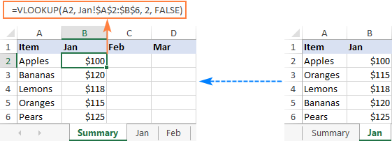
I have sheet 1 as below. What I need is similar to a VLookup where on sheet 2 it will give me whats in column B on sheet 1 when the corresponding numbers in column A are found. Problem is VLookup only returns one result for each number.

Sheet 1

Number	Number1
M14307100294003	M279
M14307100294003	M280
M14307100294003	M281
M14307100294003	M282
M14307100294003	M283

Sheet 2 Using VLookup

Number	Number1
M14307100294003	M279
M14307100294003	M279
M14307100294003	M279
M14307100294003	M279
M14307100294003	M279

Obviously on sheet 2 I would like the same result that is on sheet 1. There will be 10s of 1000s of rows and any different amount of matching numbers in column A.
Thanks.

 

[alansidman]

Here is a UDF developed by Krishnakumar. The syntax for this is MLOOKUP(TableArray,LookupValue,LookupRange,[NthMatch])

Function MLOOKUP(ByRef TableArray As Range, ByVal LookupVal, ByRef LookupRange As Range, _
                                                        Optional ByVal NthMatch As Long)

' Author        : Krishnakumar @ ExcelFox.com


If Not TypeOf TableArray Is Range Then
    MLOOKUP = CVErr(2042)
    Exit Function
End If
If Not TypeOf LookupRange Is Range Then
    MLOOKUP = CVErr(2042)
    Exit Function
End If
If TableArray.Rows.Count <> LookupRange.Rows.Count Then
    MLOOKUP = CVErr(2042)
    Exit Function
End If
If TableArray.Columns.Count <> LookupRange.Columns.Count Then
    MLOOKUP = CVErr(2042)
    Exit Function
End If

Dim LV_Cnt      As Long 'Count Loookup Value
Dim KA1, KA2
Dim r As Long, c As Long
Dim fFoundNo    As Long
Dim n           As Long
Dim strLval     As String

If IsNumeric(LookupVal) Then
    LV_Cnt = Evaluate("countif(" & LookupRange.Address & "," & LookupVal & ")")
    fFoundNo = Evaluate("match(" & CLng(LookupVal) & "," & LookupRange.Address & ",0)")
ElseIf IsDate(LookupVal) Then
    LV_Cnt = Evaluate("countif(" & LookupRange.Address & "," & CLng(LookupVal) & ")")
    fFoundNo = Evaluate("match(" & CLng(LookupVal) & "," & LookupRange.Address & ",0)")
Else
    strLval = """" & LookupVal & """"
    LV_Cnt = Evaluate("countif(" & LookupRange.Address & "," & strLval & ")")
    fFoundNo = Evaluate("match(" & strLval & "," & LookupRange.Address & ",0)")
End If

If NthMatch > 0 Then
    If LV_Cnt = 0 Or NthMatch > LV_Cnt Then
        MLOOKUP = CVErr(2042)
        Exit Function
    End If
End If


KA1 = TableArray: KA2 = LookupRange

For r = fFoundNo To UBound(KA1, 1)
    For c = 1 To UBound(KA1, 2)
        If LCase$(KA2(r, c)) = LCase$(LookupVal) Then
            If NthMatch Then
                n = n + 1
                If n = NthMatch Then
                    MLOOKUP = KA1(r, c)
                    Exit Function
                End If
            Else
                MLOOKUP = MLOOKUP & "," & KA1(r, c)
            End If
        End If
    Next
Next
MLOOKUP = Mid$(MLOOKUP, 2)
End Function

 

[Dazzawm]

Here is a UDF developed by Krishnakumar. The syntax for this is MLOOKUP(TableArray,LookupValue,LookupRange,[NthMatch])

Function MLOOKUP(ByRef TableArray As Range, ByVal LookupVal, ByRef LookupRange As Range, _
                                                        Optional ByVal NthMatch As Long)

' Author        : Krishnakumar @ ExcelFox.com


If Not TypeOf TableArray Is Range Then
    MLOOKUP = CVErr(2042)
    Exit Function
End If
If Not TypeOf LookupRange Is Range Then
    MLOOKUP = CVErr(2042)
    Exit Function
End If
If TableArray.Rows.Count <> LookupRange.Rows.Count Then
    MLOOKUP = CVErr(2042)
    Exit Function
End If
If TableArray.Columns.Count <> LookupRange.Columns.Count Then
    MLOOKUP = CVErr(2042)
    Exit Function
End If

Dim LV_Cnt      As Long 'Count Loookup Value
Dim KA1, KA2
Dim r As Long, c As Long
Dim fFoundNo    As Long
Dim n           As Long
Dim strLval     As String

If IsNumeric(LookupVal) Then
    LV_Cnt = Evaluate("countif(" & LookupRange.Address & "," & LookupVal & ")")
    fFoundNo = Evaluate("match(" & CLng(LookupVal) & "," & LookupRange.Address & ",0)")
ElseIf IsDate(LookupVal) Then
    LV_Cnt = Evaluate("countif(" & LookupRange.Address & "," & CLng(LookupVal) & ")")
    fFoundNo = Evaluate("match(" & CLng(LookupVal) & "," & LookupRange.Address & ",0)")
Else
    strLval = """" & LookupVal & """"
    LV_Cnt = Evaluate("countif(" & LookupRange.Address & "," & strLval & ")")
    fFoundNo = Evaluate("match(" & strLval & "," & LookupRange.Address & ",0)")
End If

If NthMatch > 0 Then
    If LV_Cnt = 0 Or NthMatch > LV_Cnt Then
        MLOOKUP = CVErr(2042)
        Exit Function
    End If
End If


KA1 = TableArray: KA2 = LookupRange

For r = fFoundNo To UBound(KA1, 1)
    For c = 1 To UBound(KA1, 2)
        If LCase$(KA2(r, c)) = LCase$(LookupVal) Then
            If NthMatch Then
                n = n + 1
                If n = NthMatch Then
                    MLOOKUP = KA1(r, c)
                    Exit Function
                End If
            Else
                MLOOKUP = MLOOKUP & "," & KA1(r, c)
            End If
        End If
    Next
Next
MLOOKUP = Mid$(MLOOKUP, 2)
End Function

I just get a result of VALUE, how do I use it, where to I put the formula?

 

[alansidman]

Put the formula in the cell you wish to get the results in.

MLOOKUP.xlsm
	A	B	C	D	E	F	G
1	4/1/2011	SN	181
2	4/2/2011	DC	825
3	4/3/2011	QO	512		QO		512,348,777,599
4	4/4/2011	JK	354		DC		825,394,518,509
5	4/4/2011	DC	394
6	4/4/2011	OF	921
7	4/4/2011	DC	518
8	4/4/2011	QO	348
9	4/9/2011	DC	509
10	4/10/2011	MI	193
11	4/11/2011	BA	329
12	4/12/2011	AI	930
13	4/13/2011	QO	777
14	4/14/2011	OH	962
15	4/15/2011	FS	221
16	4/16/2011	RU	419
17	4/17/2011	KU	115
18	4/18/2011	QO	599
19	4/19/2011	WJ	657
20	4/20/2011	AM	105
21	4/21/2011	WJ	786
22	4/22/2011	RN	457
23	4/23/2011	DF	343
24	4/24/2011	SN	848
25	4/25/2011	WP	956
Sheet1

Cell Formulas
Range	Formula
G3:G4	G3	=MLOOKUP($C$1:$C$25,E3,$B$1:$B$25)

 

[Dazzawm]

Put the formula in the cell you wish to get the results in.

MLOOKUP.xlsm
	A	B	C	D	E	F	G
1	4/1/2011	SN	181
2	4/2/2011	DC	825
3	4/3/2011	QO	512		QO		512,348,777,599
4	4/4/2011	JK	354		DC		825,394,518,509
5	4/4/2011	DC	394
6	4/4/2011	OF	921
7	4/4/2011	DC	518
8	4/4/2011	QO	348
9	4/9/2011	DC	509
10	4/10/2011	MI	193
11	4/11/2011	BA	329
12	4/12/2011	AI	930
13	4/13/2011	QO	777
14	4/14/2011	OH	962
15	4/15/2011	FS	221
16	4/16/2011	RU	419
17	4/17/2011	KU	115
18	4/18/2011	QO	599
19	4/19/2011	WJ	657
20	4/20/2011	AM	105
21	4/21/2011	WJ	786
22	4/22/2011	RN	457
23	4/23/2011	DF	343
24	4/24/2011	SN	848
25	4/25/2011	WP	956
Sheet1

Cell Formulas
Range	Formula
G3:G4	G3	=MLOOKUP($C$1:$C$25,E3,$B$1:$B$25)

But the results will need to be on sheet 2 and taking the info from sheet 1? This is appearing to have the info and result on same sheet which is whats confusing me.

 

[Dazzawm]

Also the results are in the same cell, I need them all downwards like in my example.

 

[Dazzawm]

Any other ideas on this please anyone?

 

[alansidman]

To get the data to display in a column tweak the formula as follows: =@MLOOKUP($C$1:$C$2200,$E$2,$B$1:$B$2200,ROWS($F$2:F12)).

change the last optional item to the section showing Rows and the range of rows.

 

[Dazzawm]

But is the result going to be on sheet 2 getting the data from sheet 1?

 

[alansidman]

You need to reference the sheet(s) where the data is located for this to happen. Look at how it happens in regular Vlookup and adapt.

VLOOKUP across multiple sheets in Excel with examples

Formula examples to Vlookup from another worksheet or workbook, Vlookup in multiple sheets, and indirect Vlookup to dynamically pull data from several worksheets into different cells.

www.ablebits.com