OK, the graph you want is similar to what I posted previously. I downloaded the data from Yahoo!Finance, eliminated all columns except for the date and closing price column. Here's a tiny excerpt. There are two columns of 345 rows. I then sorted the data from oldest to newest.
| A | B |
| 1 | Date | Close |
| 2 | 1987-12-28 | 823.2 |
| 3 | 1988-01-04 | 908.9 |
| 4 | 1988-02-01 | 888.8 |
| 5 | 1988-03-01 | 925.8 |
<tbody>
</tbody>
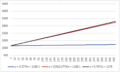
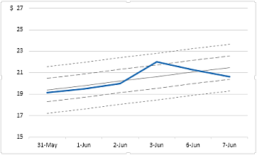
The first step is to select only B1:B345. Do not select the date column. Then insert a line chart. The x-axis labels should be a series of increasing numbers, not dates. Now insert a linear trendline and make sure the trendline equation is displayed. The equation should be very close to:
y = 5.7971x + 1178. To be like the example chart format the trendline to be small red plus signs (dots?).
Use column C as a helper column. Fill the column from C2 downward with the numbers from 1 to 344. You can use either Home >> Fill >> Series from the menu bar or use a formula.
The lines parallel to the trendline appear to be set at ±1.0 and ±1.5 times the standard deviation. These are calculated in columns D through F as shown below. The formulas in row 2 are copied downward.
| Excel 2012 |
|---|
|
|---|
| A | B | C | D | E | F | G |
|---|
| 1 | Date | Close | Helper | Tr-1.5*StDev | Tr-1*StDev | Tr+1*StDev | Tr+1.5*StDev |
|---|
| 2 | 1987-12-28 | 823.2 | 1 | 104.4102 | 464.2058 | 1903.388 | 2263.184 |
|---|
| 3 | 1988-01-04 | 908.9 | 2 | 110.2073 | 470.0029 | 1909.185 | 2268.981 |
|---|
| 4 | 1988-02-01 | 888.8 | 3 | 116.0044 | 475.8 | 1914.983 | 2274.778 |
|---|
| 5 | 1988-03-01 | 925.8 | 4 | 121.8015 | 481.5971 | 1920.78 | 2280.575 |
|---|
|
|---|
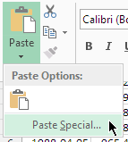
Select D1:G345 and copy the cells. Then select the chart. With the chart selected, go to the Home tab on the ribbon. Under the Clipboard Paste icon is a small downward pointing triangle. Click the triangle, then select "Paste Special".
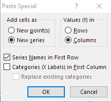
In the dialog box that pops up, select "New Series", "Columns", "Series Names in First Row" and then press "OK",
The standard deviation lines should appear in the chart.
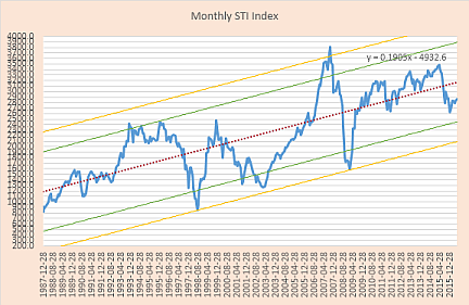
Now we'll make the x-axis show dates instead of numbers. Select the chart and right-click to bring up the pop-up menu. Choose "Select data". In the dialog box that pops up, click on the right-hand "Edit" button. In the "Axis Labels" dialog box, enter "A2:A345". Press "OK" in that dialog box, then press "OK" in the "Select Data Source" dialog box and you should be returned to your chart, now showing dates on the x-axis.
The remainder is just formatting. The chart area is a light orange; the plot area is white; the y-axis is set to run from 200 to 4000 with 100 points as the interval; the x-axis has an 8-month interval; and so on. Too busy for my taste but it matches your example.
![CzUDCWk]](/board/proxy.php?image=http%3A%2F%2F%5Bhttp%3A%2F%2Fimgur.com%2FCzUDCWk%5D&hash=05dfcdda00bfadab20f599bead5f8f29)
![0ZDC9yP]](/board/proxy.php?image=http%3A%2F%2F%5Bhttp%3A%2F%2Fimgur.com%2F0ZDC9yP%5D&hash=97029bacfcbe5d2e345b8fc2c6501e5c)