Sum first n cells

raikks

Board Regular
Joined
Feb 23, 2020
Messages
53
Office Version
  1. 2019
Platform
  1. Windows
Hi - I need a formula that sums the first 3 cells of component1 that contains ``yes'' (result should be 88)
Also - I need to sum the first 3 cells of component1 & component2 that contains ``yes'' (result should be 121)
Thanks in advance.
 

Attachments

  • Untitled.png
    Untitled.png
    4.8 KB · Views: 17

Excel Facts

Can you AutoAverage in Excel?
There is a drop-down next to the AutoSum symbol. Open the drop-down to choose AVERAGE, COUNT, MAX, or MIN
Hi,

Welcome to the Board!

Please test the following formula:

=SUMIF(A2:INDEX(A:A,SMALL(IF(A:A="yes",1,1000)*ROW(A:A),3)),"Yes",C2:INDEX(C:C,SMALL(IF(A:A="yes",1,1000)*ROW(A:A),3)))
You have to confirm it using Ctrl-Shift-Enter.
 
Upvote 0
First one:

=SUMIF(A2:INDEX(A2:A10,AGGREGATE(15,6,(ROW(A2:A10)-ROW(A2)+1)/(A2:A10="yes"),3)),"yes",C2:C10)

Have to go. Will come back to the second one later if not resolved.
 
Upvote 0
Hi,

Welcome to the Board!

Please test the following formula:

=SUMIF(A2:INDEX(A:A,SMALL(IF(A:A="yes",1,1000)*ROW(A:A),3)),"Yes",C2:INDEX(C:C,SMALL(IF(A:A="yes",1,1000)*ROW(A:A),3)))
You have to confirm it using Ctrl-Shift-Enter.
Jesus - it works!
Thank you, sir!
 
Upvote 0
First one:

=SUMIF(A2:INDEX(A2:A10,AGGREGATE(15,6,(ROW(A2:A10)-ROW(A2)+1)/(A2:A10="yes"),3)),"yes",C2:C10)

Have to go. Will come back to the second one later if not resolved.
Thank you, it works!
Would very much appreciate a solution for the second one as well.
 
Upvote 0
Thank you, it works!
Would very much appreciate a solution for the second one as well.
Does the double "Yes" in the first row count as 2 or as 1 "Yes"?
 
Upvote 0
I think it counts as 1 ``yes''.
I'll attach another pic to emphasize what I really want to sum up.
Let me know if it's clear.
 

Attachments

  • Untitled2.png
    Untitled2.png
    5.6 KB · Views: 9
Upvote 0
Second one:

If you use a helper cell (G1 for me) with this formula:
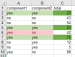
=AGGREGATE(15,6,ROW(C2:C10)/((A2:A10="yes")*(B2:B10="yes")),3)
then
=SUMIFS(C2:INDEX(C:C,G1),A2:INDEX(A:A,G1),"yes",B2:INDEX(B:B,G1),"yes")


If you want without a helper then ..
=SUMIFS(C2:INDEX(C:C,AGGREGATE(15,6,ROW(C2:C10)/((A2:A10="yes")*(B2:B10="yes")),3)),A2:INDEX(A:A,AGGREGATE(15,6,ROW(C2:C10)/((A2:A10="yes")*(B2:B10="yes")),3)),"yes",B2:INDEX(B:B,AGGREGATE(15,6,ROW(C2:C10)/((A2:A10="yes")*(B2:B10="yes")),3)),"yes")
 
Upvote 0
OK, here you go:
=SUMIFS(C2:INDEX(C:C,SMALL(IF((A:A="yes")+(B:B="yes")=2,1,1000)*ROW(A:A),3)), A2:INDEX(A:A,SMALL(IF((A:A="yes")+(B:B="yes")=2,1,1000)*ROW(A:A),3)),"Yes", B2:INDEX(B:B,SMALL(IF((A:A="yes")+(B:B="yes")=2,1,1000)*ROW(A:A),3)),"Yes")
Again use Ctrl-Shift-Enter.
 
Upvote 0
Thank you once again - extremely helpful for me this formula.
 
Upvote 0

Forum statistics

Threads
1,212,927
Messages
6,110,733
Members
448,294
Latest member
jmjmjmjmjmjm

We've detected that you are using an adblocker.

We have a great community of people providing Excel help here, but the hosting costs are enormous. You can help keep this site running by allowing ads on MrExcel.com.
Allow Ads at MrExcel

Which adblocker are you using?

Disable AdBlock

Follow these easy steps to disable AdBlock

1)Click on the icon in the browser’s toolbar.
2)Click on the icon in the browser’s toolbar.
2)Click on the "Pause on this site" option.
Go back

Disable AdBlock Plus

Follow these easy steps to disable AdBlock Plus

1)Click on the icon in the browser’s toolbar.
2)Click on the toggle to disable it for "mrexcel.com".
Go back

Disable uBlock Origin

Follow these easy steps to disable uBlock Origin

1)Click on the icon in the browser’s toolbar.
2)Click on the "Power" button.
3)Click on the "Refresh" button.
Go back

Disable uBlock

Follow these easy steps to disable uBlock

1)Click on the icon in the browser’s toolbar.
2)Click on the "Power" button.
3)Click on the "Refresh" button.
Go back
Back
Top