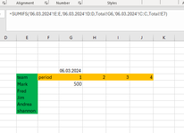
I am working on a sheet to track OT cost, I have a total page that has all the teams and months(periods), and extracts data from report that are save as sheet with date format. Currently I have =sumifs('06.03.2024'!F:F,'06.03.2024'!A:A,'06.03.2024'!B:B,N3) I would like it so that the 06.03.2024 is replaced with the cell(G6) it is in this way I can just copy the formula over and not have to go and change the date in formula every time I do a update for the next period. looking for something like this sumifs('b$1'!$F:$F,'$b1'!$A:$A,'$b1'!$B:$B,$N3) next period sumifs('c$1'!$F$:F,'c$1'!$A:$A,'c$1'!$B:$B,N$3) and so on. I have attempted indirect but not working. I might be missing something. thanks in advance.
-
If you would like to post, please check out the MrExcel Message Board FAQ and register here. If you forgot your password, you can reset your password.
sum formula, using cell to refer to sheet name.
- Thread starter NickYOW
- Start date