Sum if columns match in separate sheets and total from another column

[2k05gt]

I have been hurting my brain on this..
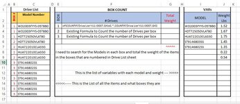
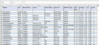
I have 3 sheets, 1 sheet "VARs" is a List of the items specs by Model Number, the column I need to sum is in this case weight in Lbs
Sheet 2 "Drive_List" is a List of items that have the same model number (S/N make the different) that are put into Boxes that are numbered
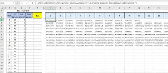
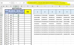
Sheet 3 is "Box Count" this is a count of how many items are in a box and how much it weights . Here is the issue.
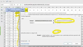
How can I get a sum of all the items weight in each box. the weight of each item (model number) is different and each box has a mix of the items.

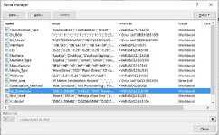
I tried using indexing, with offset but working with 3 different sheets got confusing, I defined names for each of the columns I was working with
but nothing would work.

Thanks in advance for any assistance

 

[KRice]

Some notional data:

Book1
	A	B	C
1		Model	Weight (lb)
2		a	2
3		b	1.75
4		c	1.5
5		d	1
6		e	1.25
7		f	0.75
VARS

Book1
	A	B	C
1		Box #	Model
2		1	a
3		1	a
4		1	b
5		2	a
6		2	a
7		2	b
8		2	c
9		2	c
10		3	b
11		3	b
12		3	c
13		4	a
14		4	c
Drive_List

Then for the summary:

Book1
	A	B	C	D	E
1		Box	# Drives	Total Weight	Items in Box
2		1	3	5.75	a, a, b
3		2	5	8.75	a, a, b, c, c
4		3	3	5	b, b, c
5		4	2	3.5	a, c
BOX COUNT

Cell Formulas
Range	Formula
C2:C5	C2	=COUNTIF(Drive_List!$B$2:$B$14,B2)
D2:D5	D2	=SUM(XLOOKUP(FILTER(Drive_List!$C$2:$C$14,Drive_List!$B$2:$B$14=B2),VARS!$B$2:$B$7,VARS!$C$2:$C$7))
E2:E5	E2	=TEXTJOIN(", ",,FILTER(Drive_List!$C$2:$C$14,Drive_List!$B$2:$B$14=B2))

 

[2k05gt]

Thanks for the Reply, I do not have XLookup, TextJoin or Filter Functions I am using 2016 I think

 

[KRice]

I would have sworn I saw 365 in your profile
Without the 365 functions, the job is a little more difficult, and you will benefit from using some helper columns to tabulate the models found in each box. See the green-shaded section to the right. Pull those formulas out to the right until you see blanks, which means you've covered all items in that box. If you do this once for the maximum number of drives expected to ever be found in a box, then you shouldn't have to do it again.

Book1
	A	B	C	D	E	F	G	H	I	J	K	L	M	N	O	P
1		Box	# Drives	Total Weight				Helper Area
2		1	3	5.75				a	a	b
3		2	5	8.75				a	a	b	c	c
4		3	3	5				b	b	c
5		4	2	3.5				a	c
BOX COUNT

Cell Formulas
Range	Formula
C2:C5	C2	=COUNTIF(Drive_List!$B$2:$B$14,B2)
D2:D5	D2	=SUM(SUMIF(VARS!$B$2:$B$7,$H2:INDEX(H2:ZZ2,,C2),VARS!$C$2:$C$7))
H2:O5	H2	=IF(COLUMNS($D:D)<=$C2,INDEX(Drive_List!$C:$C,AGGREGATE(15,6,ROW(Drive_List!$B$2:$B$14)/(Drive_List!$B$2:$B$14=$B2),COLUMNS($D:D))),"")

If you want to simplify the SUMIF formula, you could replace the dynamically formed range $H2:INDEX(H2:ZZ2,,C2) with the maximum range of your helper cells...for example H2:O2...so the formula would be:

=SUM(SUMIF(VARS!$B$2:$B$7,H2:O2,VARS!$C$2:$C$7))

 

[2k05gt]

Not sure what's it not picking up, but the weight shows Zero

 

[KRice]

Would you show the formula being used in the cell that is producing 0?

 

[2k05gt]

Would you show the formula being used in the cell that is producing 0?

 

[KRice]

Have a look again at how that dynamically formed range is constructed in the SUMIF function. I believe you want:

$H3:INDEX(H3:ZZ3,,C3)

...you have an extra :$AK3: in the expression.

 

[2k05gt]

Have a look again at how that dynamically formed range is constructed in the SUMIF function. I believe you want:

$H3:INDEX(H3:ZZ3,,C3)

...you have an extra :$AK3: in the expression.

Still shows as 0 but when viewed in formula results it looks correct

 

[KRice]

Ok...good. You can see the array in your diagnostics. Click on the cell with the formula, then go into the formula bar where the formula appears (click at the end of the formula), and re-confirm the entry by entering it with Ctrl-Shift-Enter, to enter the formula as an array formula. You should see curly brackets form around the expression. Alternatively, replace this dynamically formed array with a simple range reference to the helper cells in that row.