SUM Substitution

DTal2076

New Member
Joined
Dec 28, 2020
Messages
4
Office Version
  1. 365
Platform
  1. Windows
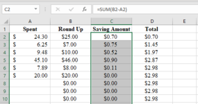
I am trying to create a spread that will provide me with a round up savings total since my bank does not offer that feature. I would like to insert my debit amount, round it up to the next dollar amount, deduct the debit from the rounded amount, and total the differences so I can transfer that total to my savings account at the end of the month/quarter. When I have a flat dollar amount, $20, it rounds that to $20 dollars. Making the difference to be added to the total savings column $0. Could one of you kind folks help me create a formula that would substitute that $0 dollar SUM with $1. In case my description sucks, I have provided a picture with what I have so far.
 

Attachments

  • Capture.PNG
    Capture.PNG
    17.8 KB · Views: 10

Excel Facts

Is there a shortcut key for strikethrough?
Ctrl+S is used for Save. Ctrl+5 is used for Strikethrough. Why Ctrl+5? When you use hashmarks to count |||| is 4, strike through to mean 5.
You can do this with the RoundUp function and just subtracting the spent value from the roundUp value. Then for the running total do =SUM($C$2:C2).

But, to avoid having to drag the formulas down and have a bunch of rows with zeros in them, you could use Power Query like this and only have to worry about adding items in the 'Spent' column.

Book1
ABCD
1SpentRoundUpToSavingsTotal
2$24.30 $25.00$0.70$0.70
3$6.25 $7.00$0.75$1.45
4$9.48 $10.00$0.52$1.97
5$45.10 $46.00$0.90$2.87
6$7.89 $8.00$0.11$2.98
7$20.00 $20.00$0.00$2.98
Sheet2


Power Query:
let
    Source = Excel.CurrentWorkbook(){[Name="Table1"]}[Content],
    RoundUp = Table.AddColumn(Source, "RoundUp", each Number.RoundUp([Spent],0)),
    Savings = Table.AddColumn(RoundUp, "ToSavings", each [RoundUp]-[Spent]),
    Index = Table.AddIndexColumn(Savings, "Index", 1, 1),
    Total = Table.AddColumn(Index, "Total", each List.Sum(List.FirstN(Index[ToSavings],[Index]))),
    Select = Table.SelectColumns(Total,{"RoundUp", "ToSavings", "Total"}),
    Types = Table.TransformColumnTypes(Select,{{"RoundUp", Currency.Type}, {"ToSavings", Currency.Type}, {"Total", Currency.Type}})
in
    Types
 
Upvote 0
Welcome to the Forum!

You can round up to the dollar using either:
=ROUNDUP(A1,0)
or
=CEILING(A1,1)
 
Upvote 0
You can do this with the RoundUp function and just subtracting the spent value from the roundUp value. Then for the running total do =SUM($C$2:C2).

But, to avoid having to drag the formulas down and have a bunch of rows with zeros in them, you could use Power Query like this and only have to worry about adding items in the 'Spent' column.

Book1
ABCD
1SpentRoundUpToSavingsTotal
2$24.30 $25.00$0.70$0.70
3$6.25 $7.00$0.75$1.45
4$9.48 $10.00$0.52$1.97
5$45.10 $46.00$0.90$2.87
6$7.89 $8.00$0.11$2.98
7$20.00 $20.00$0.00$2.98
Sheet2


Power Query:
let
    Source = Excel.CurrentWorkbook(){[Name="Table1"]}[Content],
    RoundUp = Table.AddColumn(Source, "RoundUp", each Number.RoundUp([Spent],0)),
    Savings = Table.AddColumn(RoundUp, "ToSavings", each [RoundUp]-[Spent]),
    Index = Table.AddIndexColumn(Savings, "Index", 1, 1),
    Total = Table.AddColumn(Index, "Total", each List.Sum(List.FirstN(Index[ToSavings],[Index]))),
    Select = Table.SelectColumns(Total,{"RoundUp", "ToSavings", "Total"}),
    Types = Table.TransformColumnTypes(Select,{{"RoundUp", Currency.Type}, {"ToSavings", Currency.Type}, {"Total", Currency.Type}})
in
    Types
I understand all of that and referencing my picture and your picture the problem still is not resolved. C7 is still zero. Is there a way to take a sum of zero and replace it with 1 via an IF function, SUB function, or SUBIF function?
 
Upvote 0
I am not sure exactly what you require.
Try
T202012c.xlsm
A
1Amount
224.30
36.25
49.48
545.10
67.89
720.00
8113.02
92.98
2c
Cell Formulas
RangeFormula
A8A8=SUM(A2:A7)
A9A9=SUMPRODUCT(ROUNDUP(A2:A7,0)-A2:A7)
 
Upvote 0
With your latest information. Try either the total or detail.
T202012c.xlsm
ABC
1AmountRoundupDifference
224.3025.000.70
36.257.000.75
49.4810.000.52
545.1046.000.90
67.898.000.11
720.0021.001.00
8113.02117.003.98
93.98
2c
Cell Formulas
RangeFormula
B2:B6B2=ROUNDUP(A2,0)
C2:C7C2=B2-A2
B7B7=ROUNDUP(A7,0)+(ROUNDUP(A7,0)=A7)
A8:C8B8=SUM(B2:B7)
A9A9=SUMPRODUCT(ROUNDUP(A2:A7,0)-A2:A7+(ROUNDUP(A2:A7,0)=A2:A7))
 
Last edited:
Upvote 0
Book1
ABCD
1SpentRoundUpToSavingsTotal
2$24.30 $25.00$0.70$0.70
3$6.25 $7.00$0.75$1.45
4$9.48 $10.00$0.52$1.97
5$45.10 $46.00$0.90$2.87
6$7.89 $8.00$0.11$2.98
7$20.00 $21.00$1.00$3.98
Sheet2


Power Query:
let
    Source = Excel.CurrentWorkbook(){[Name="Table1"]}[Content],
    RoundUp = Table.AddColumn(Source, "RoundUp", each if Int64.From([Spent])-[Spent] = 0 then Number.RoundUp([Spent],0)+1 else Number.RoundUp([Spent],0)),
    Savings = Table.AddColumn(RoundUp, "ToSavings", each [RoundUp]-[Spent]),
    Index = Table.AddIndexColumn(Savings, "Index", 1, 1),
    Total = Table.AddColumn(Index, "Total", each List.Sum(List.FirstN(Index[ToSavings],[Index]))),
    Select = Table.SelectColumns(Total,{"RoundUp", "ToSavings", "Total"}),
    Types = Table.TransformColumnTypes(Select,{{"RoundUp", Currency.Type}, {"ToSavings", Currency.Type}, {"Total", Currency.Type}})
in
    Types
 
Upvote 0
Upvote 0

Forum statistics

Threads
1,215,407
Messages
6,124,723
Members
449,184
Latest member
COrmerod

We've detected that you are using an adblocker.

We have a great community of people providing Excel help here, but the hosting costs are enormous. You can help keep this site running by allowing ads on MrExcel.com.
Allow Ads at MrExcel

Which adblocker are you using?

Disable AdBlock

Follow these easy steps to disable AdBlock

1)Click on the icon in the browser’s toolbar.
2)Click on the icon in the browser’s toolbar.
2)Click on the "Pause on this site" option.
Go back

Disable AdBlock Plus

Follow these easy steps to disable AdBlock Plus

1)Click on the icon in the browser’s toolbar.
2)Click on the toggle to disable it for "mrexcel.com".
Go back

Disable uBlock Origin

Follow these easy steps to disable uBlock Origin

1)Click on the icon in the browser’s toolbar.
2)Click on the "Power" button.
3)Click on the "Refresh" button.
Go back

Disable uBlock

Follow these easy steps to disable uBlock

1)Click on the icon in the browser’s toolbar.
2)Click on the "Power" button.
3)Click on the "Refresh" button.
Go back
Back
Top