SumColor not working after applying Additional Formatting

[KXZ]

I'm not very savy with excel but I manage to figure most stuff out but I am having a hard time trying figure out how to sum by color with conditional formatting.

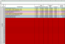
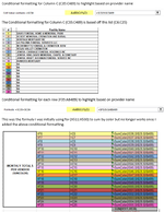
I have a column of invoice amounts that I need to total the amounts by color. My rows are formatted to highlight a specific color when I enter a provider name.

I found a way to sum by color but it only worked for cells whose color was set manually not using conditional formatting. Once conditional formatting was applied this method no longer worked.

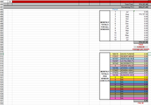
X511:X530 (20 cells) for each provider total, Range is X35:X489

Any help would be greatly appreciated, thank you.

 

[6StringJazzer]

You need to use the same logic to calculate the sum as you are using for your conditional formatting rule.

I am not seeing "a column of invoice amounts" in your screen shot. What does that look like?

What is your conditional formatting rule?

 

[KXZ]

You need to use the same logic to calculate the sum as you are using for your conditional formatting rule.

I am not seeing "a column of invoice amounts" in your screen shot. What does that look like?

What is your conditional formatting rule?

The first image is for the invoice column with the range of X35:X489

Second image are the formatting rules

 

[6StringJazzer]

You don't need to sum by color at all because you have the facility name on each invoice line. Sum like this in Y511 and copy down to Y530:

=SUMIF(C35:C489, X511, X35:X489)

 

[KXZ]

You don't need to sum by color at all because you have the facility name on each invoice line. Sum like this in Y511 and copy down to Y530:

=SUMIF(C35:C489, X511, X35:X489)

Thank you! that worked.

 

[6StringJazzer]

One error. Ranges need to be absolute to be able to copy down,

=SUMIF(C$35:C$489, X511, X$35:X$489)