rsd007
New Member
- Joined
- Oct 24, 2022
- Messages
- 27
- Office Version
- 2019
- Platform
- Windows
Hello,
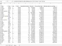
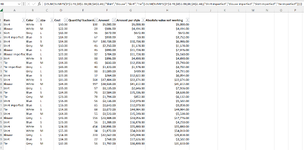
i am working on a task to calculate total value of product in Excel with multiple criteria and my formula of SUMIFS not working as the amounts are some +ve and some -ve so trying to do SUMIFS with absolute value base on each category, style various sizes as well as backorder and imperfect product. Hoping some one can help me out.
Thanks
For the help
Formula used in G 2 is =SUM(SUMIFS($F$2:F2, $B$2:B2,B2,$A$2:A2, {"Shirt","Blouse","Skirt","Tie"}))
and Formula used in H 2 is =SUM(SUMIFS($F$1:F2,$B$1:B2,B2,$A$1:A2,{"Shirt","Blouse","Skirt","Tie"})-SUM(SUMIFS($F$1:F2,$B$1:B2,B2,$A$1:A2,{"Shirt imperfect","Blouse imperfect","Skirt imperfect","Tie imperfect"})))