Table with a column for due dates and color changes per time

[cmz3]

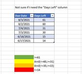
I have several client tabs with tables and each table has a column for due dates. How do I change the change the color based on the time left from today? I was able to conditional format one cell but unlike formulas in a table it didn't transfer to all cells in the column. I currently have 4 tabs with over 100 cells each that need to be formatted. This would take forever doing a conditional format on each one. Any ideas?

 

[Joe4]

I was able to conditional format one cell but unlike formulas in a table it didn't transfer to all cells in the column.

The best way I have found to do Conditional Formatting on a large range is to select ALL the cells you want to apply it to from the start.
Then, write the Conditional Formatting formula as it applies to the very first cell in your selection, and it should adjust it automatically for all the others in your selection.

If you are still having issues, post the Conditional Formatting rule/formula you are using, and a sample of your data and expected results.

 

[cmz3]

That didn't work. It changed all cells in the column just based on the 1st cell. Maybe because I have a formatted Table rather than just plain table?

 

[cmz3]

Please see below. This is what I am trying to do.

 

[Joe4]

That didn't work. It changed all cells in the column just based on the 1st cell. Maybe because I have a formatted Table rather than just plain table?

If you have multiple columns that you want to be formatted based on the value in one column, you usually need to lock that column down through the use of Absolute/Mixed cell references (see: Absolute, Relative, and Mixed Cell References in Excel).

So if you wanted both columns B and C in row 2 formatted based on the value of column C, the formula would look like:
=$C2>=61
as you want the column to be "fixed" at column C, but want the rows to "float" so it will work for other rows.