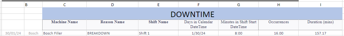
hi all - how can I expand on Fluff's formula to include to return the same ranges only if column E contains the text "shift 1"?
=TAKE(SORT(HSTACK(i43:i1501,d43:d1501),1,-1),5)
so still looks at top 5 times in column I
matches the times to the reason code in column D
but only gets the top 5 times for the text "shift 1" from column E
TIA
=TAKE(SORT(HSTACK(i43:i1501,d43:d1501),1,-1),5)
so still looks at top 5 times in column I
matches the times to the reason code in column D
but only gets the top 5 times for the text "shift 1" from column E
TIA