tattslotto spread sheet

[Grahamscown]

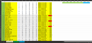
I have a spreadsheet columns A to J and rows 1 to 250 that contain the syndicate data and cells N2 to U2 that i will input the weekly drawn 6 numbers and 2 supps
1I need the numbers in columns C to H to turn green for the weekly drawn numbers and blue for the supps entered entered into cells N2 to U2 Im not sure how to upload the file so i will upload an image of the spread sheet

 

[mumps]

Do a little research into using conditional formatting.

 

[Grahamscown]

Hi sorry but not knowing much about the subject or the terminology makes it very hard I cant use duplicate values because it highlights every cell I need the cells IN COLUMNS C TO H to highlight only when the numbers are entered into N2 TO U2

 

[mumps]

It is hard to work with a picture. It would be easier to help if you could use the XL2BB add-in (icon in the menu) to attach a screenshot (not a picture) of your sheet. Alternately, you could upload a copy of your file to a free site such as www.box.com or www.dropbox.com. Once you do that, mark it for 'Sharing' and you will be given a link to the file that you can post here. Explain in detail what you want to do referring to specific cells, rows, columns and sheets using a few examples from your data (de-sensitized if necessary).

 

[Grahamscown]

SHARE HOLDERS.xlsx

Shared with Dropbox

www.dropbox.com

 

[mumps]

Select the range from C2:H70 and use the following formulas in your conditional formatting:
blue:

=OR(C2=$T$2,C2=$U$2)

green:

=OR(C2=$N$2,C2=$O$2,C2=$P$2,C2=$Q$2,C2=$R$2,C2=$S$2)

You have to of course select the fill colour for each one.

 

[Grahamscown]

Select the range from C2:H70 and use the following formulas in your conditional formatting:
blue:

=OR(C2=$T$2,C2=$U$2)

green:

=OR(C2=$N$2,C2=$O$2,C2=$P$2,C2=$Q$2,C2=$R$2,C2=$S$2)

You have to of course select the fill colour for each one.

Thankyou i was nervous about trying your fix first but found it easy enough to do and very understandable and most of all it worked exactly as i wanted it to Thankyou again

 

[mumps]

You are very welcome.