Tiered commission excel formula problem

[Zancia]

Hi all,



I see you are all very helpful in this forum, so maybe you will help me to find solution to this one.

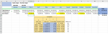
I have to find the right formula to calculate monthly commissions for the sales made in the month but based on the annual target.



For sales up to 60000 in a year, no commission

Sales between 60001 and 120000, 10% of the sales in the month

Total sales between 120001-180000, 15% of what has been brought in

Total sales between 180001-240000, 25% of the amount brought in



I used vlookup and sumproduct but something went wrong.

It complicates when i.e. total sales in previous month were 95000 and then in the next month SP brings in 75000, total sales are then 170000

If I use vlookup or sumproduct it will take whole 75000 @ 15% because total sales are more than 120000 and I would need this to be divided to 25000 @ 10% (in the range 60001-120000) and 50000 @ 15% (120001-180000).



How can I do it? Any advice would be much appreciated.

Thank you

 

[arthurbr]

Check McGimpsey & Associates : Excel : How differential rates work

 

[Zancia]

Hi All,
It is me again still with the same problem after almost a year.
Can anyone please advise on formula for tiered commissions where we take into consideration the annual sales but give commission only of what has been brought in in each month?
below are the tiers for annual sales :

Sales Tiers	Sales min	Comm Rate
0 - 48000	€ 0.00	0.0%
48001 - 132000	€ 48,000.00	10.0%
132001 - 192000	€ 132,000.00	15.0%
192001 - 250000	€ 192,000.00	20.0%
250001 - 300000	€ 250,000.00	25.0%
Above 300,001	€ 300,000.00	30.0%

Let say that a sales person has brought in €20000 sales in first month, they get nothing but next month they brought in €50000, so the total is already 70k, but we should only give them commission on the difference 70-48=22k @ 10%. after that they bring in 100k which gives a total of 170k sales so they should be getting commission on 100k (170-132 = 38 @ 15% and 62k @ 10%). Can anyone help with creating this formula?
I used VLOOKUP and SUMPRODUCT but I guess it is more complicated than I thought.

D7: =VLOOKUP(D6,$F$13:$G$18,2,TRUE)*D5

Thank you in advance for your help!

and ps. @arthurbr - I looked at the link you shared but it didn't help me much.

 

[MARK858]

Can you please post your data using the boards XL2BB addin (click the XL2BB icon in the reply window which is a link to the download and the instructions) as we can't copy and paste into Excel from an image.
Is row 7 the results that you are looking for?

 

[Zancia]

Can you please post your data using the boards XL2BB addin (click the XL2BB icon in the reply window which is a link to the download and the instructions) as we can't copy and paste into Excel from an image.
Is row 7 the results that you are looking for?

Hi, thanks for replying. The results highlighted in yellow are incorrect as the formula calculates them wrong.
I am sorry I am new in this, so I am not sure how to add the XL2BB to my excel, I tried downloading but it doesn't work.
D7 should calculate commission on 4000 from 20000 brought in only, as only 4000 exceeded the minimum threshold of 48000. So there should be 400 commission as a result in D7.
H7 should split commission on sales of 32000 to 16000 @ 15% and 16000 @ 10% = 4000
k7 should split commission on sales of 38000 to 24000 @ 20% and 14000 @ 15% = 6900

January

February

March

April

May

June

July

August

September

October

November

December

Total Money in

€12,000.00​

€20,000.00​

€20,000.00​

€24,000.00​

€28,000.00​

€12,000.00​

€32,000.00​

€10,000.00​

€20,000.00​

€38,000.00​

€26,000.00​

€20,000.00​

YTD Money in

€12,000.00​

€32,000.00​

€52,000.00​

€76,000.00​

€104,000.00​

€116,000.00​

€148,000.00​

€158,000.00​

€178,000.00​

€216,000.00​

€242,000.00​

€262,000.00​

Commission

€0.00​

€0.00​

€2,000.00​

€2,400.00​

€2,800.00​

€1,200.00​

€4,800.00​

€1,500.00​

€3,000.00​

€7,600.00​

€5,200.00​

€5,000.00​

Formula in D7: =VLOOKUP(D6,$F$13:$G$18,2,TRUE)*D5
Formula in H7: =VLOOKUP(H6,$F$13:$G$18,2,TRUE)*H5
Formula in k7: =VLOOKUP(K6,$F$13:$G$18,2,TRUE)*K5

Thanks in advance for all your help.

 

[AlanY]

is this works for you?

Book1
	A	B	C	D	E	F	G	H	I	J	K	L	M
1	Sales Tiers	Sales min	Comm Rate	Commission
2	0 - 48000	€ 0.00	0.00%	0%
3	48001 - 132000	€ 48,000.00	10.00%	10%
4	132001 - 192000	€ 132,000.00	15.00%	5%
5	192001 - 250000	€ 192,000.00	20.00%	5%
6	250001 - 300000	€ 250,000.00	25.00%	5%
7	Above 300,001	€ 300,000.00	30.00%	5%
8
9		January	February	March	April	May	June	July	August	September	October	November	December
10	Total Money in	€ 12,000.00	€ 20,000.00	€ 20,000.00	€ 24,000.00	€ 28,000.00	€ 12,000.00	€ 32,000.00	€ 10,000.00	€ 20,000.00	€ 38,000.00	€ 26,000.00	€ 20,000.00
11	YTD Money in	€ 12,000.00	€ 32,000.00	€ 52,000.00	€ 76,000.00	€ 104,000.00	€ 116,000.00	€ 148,000.00	€ 158,000.00	€ 178,000.00	€ 216,000.00	€ 242,000.00	€ 262,000.00
12	Commission	€ 0.00	€ 0.00	€ 400.00	€ 2,400.00	€ 2,800.00	€ 1,200.00	€ 4,000.00	€ 1,500.00	€ 3,000.00	€ 6,900.00	€ 5,200.00	€ 4,600.00
167

Cell Formulas
Range	Formula
D3:D7	D3	=C3-C2
C12:M12	C12	=SUMPRODUCT(--(C11>$B$2:$B$7),C11-$B$2:$B$7,$D$2:$D$7)-SUM($B$12:B12)

 

[Zancia]

is this works for you?

Book1
	A	B	C	D	E	F	G	H	I	J	K	L	M
1	Sales Tiers	Sales min	Comm Rate	Commission
2	0 - 48000	€ 0.00	0.00%	0%
3	48001 - 132000	€ 48,000.00	10.00%	10%
4	132001 - 192000	€ 132,000.00	15.00%	5%
5	192001 - 250000	€ 192,000.00	20.00%	5%
6	250001 - 300000	€ 250,000.00	25.00%	5%
7	Above 300,001	€ 300,000.00	30.00%	5%
8
9		January	February	March	April	May	June	July	August	September	October	November	December
10	Total Money in	€ 12,000.00	€ 20,000.00	€ 20,000.00	€ 24,000.00	€ 28,000.00	€ 12,000.00	€ 32,000.00	€ 10,000.00	€ 20,000.00	€ 38,000.00	€ 26,000.00	€ 20,000.00
11	YTD Money in	€ 12,000.00	€ 32,000.00	€ 52,000.00	€ 76,000.00	€ 104,000.00	€ 116,000.00	€ 148,000.00	€ 158,000.00	€ 178,000.00	€ 216,000.00	€ 242,000.00	€ 262,000.00
12	Commission	€ 0.00	€ 0.00	€ 400.00	€ 2,400.00	€ 2,800.00	€ 1,200.00	€ 4,000.00	€ 1,500.00	€ 3,000.00	€ 6,900.00	€ 5,200.00	€ 4,600.00
167

Cell Formulas
Range	Formula
D3:D7	D3	=C3-C2
C12:M12	C12	=SUMPRODUCT(--(C11>$B$2:$B$7),C11-$B$2:$B$7,$D$2:$D$7)-SUM($B$12:B12)

This is perfect. thank you so much

 

[AlanY]

you're welcome