Tiered commission formula

[dip694]

I am trying to create a spreadsheet to calculate the tentative commission for a real estate business. The commission is structured in a tiered way under two situation.
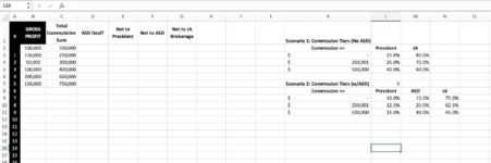
Scenario 1 - Under this scenario the brokerage president is the one that handled the sale. The split would as seen from the screenshot below: Scenario 1: Commission Tiers. This assumes that no other ASD (ie sales guy was involved).

Scenario 2 - Under this scenario, the sale was predominantly handled by the ASD (ie sales guy) while managed by the president. As such the commission tier/structure would be as outlined in Scenario 2.

My question, is what is the best formula to calculate the commission for the president, ASD, and JA (company)?

I very much appreciate all your help.

 

[Dave Patton]

I show 3 alternatives ways to calculate the commission for scenario 1 ASD = y.
The array of Bracket information is named aB and the array of Rate differentials is named aR. See E2
The named arrays are aB ={0;250000;500000}} and aR ={0.15;0.1;0.15}
The Table is not required.

If you want to use the table of brackets and rates, see F2

The same logic applies for scenario 2.
To try the suggestion below, click on the icon below the f(x) in the header and paste the information into an empty sheet.
N.B. You can post an extract of your sheet with the forum's tool XL2BB.

Commissions 2021.xlsm
	A	B	C	D	E	F	G	H	I	J	K
1				Total sales	800,000.00			Commission
2				Commission	220,000.00	220,000.00
3				Commission Arithmetic	220,000.00
4
5
6								Brackets S1	Rates		Arthmetic
7
8								0	15%		37,500
9								250,000	25%		62,500
10								500,000	40%		120,000
11				ASD
12			800,000	y	220000
2c

Cell Formulas
Range	Formula
F2	F2	=SUMPRODUCT(--(E1>H8:H10),E1-H8:H10,I8:I10-I7:I9)
E2	E2	=SUMPRODUCT(--(E1>aB),E1-aB,aR)
E3	E3	=SUM(K8:K10)
K8:K9	K8	=MAX(0,MIN($E$1,H9)-H8)*I8
K10	K10	=MAX(0,MIN($E$1,K11)-H10)*I10
E12	E12	=IF(D12="y",SUMPRODUCT(--(E1>aB),E1-aB,aR),IF(D12="","Balance of Formula",""))

 

[Dave Patton]

Information posted for the arithmetic part was not complete.
The BigNum is a named value for an extremely large number =9.99999999999999E+307

See below

Commissions 2021.xlsm
	H	I	J
6	Brackets S1	Rates	Arthmetic
7
8	0	15%	37,500
9	250,000	25%	62,500
10	500,000	40%	120,000
11	1E+308
2c

Cell Formulas
Range	Formula
J8:J10	J8	=MAX(0,MIN($E$1,H9)-H8)*I8
H11	H11	=BigNum

 

[dip694]

Thank you for your reply, but not sure I quite understand the solution. Here is an extract of my worksheet:

Commission Split.xlsx
	A	B	C	D	E	F	G	H	I	J	K	L	M	N
1	#	GROSS PROFIT	Total Cummulative Sum	ASD Deal?	Net to President	Net to ASD	Net to JA Brokerage
2		100,000	100,000	Yes							SCENARIO 1: Commission Tiers (No ASD)
3	1	150,000	250,000	No							Commission >=	President	JA
4	2	50,000	300,000	Yes							$ -	15.0%	85.0%
5	3	100,000	400,000	Yes							$ 250,001	25.0%	75.0%
6	4	200,000	600,000	No							$ 500,000	40.0%	60.0%
7	5	150,000	750,000	No
8	6										SCENARIO 2: Commission Tiers (w/ASD)
9	7										Commission >=	President	ASD	JA
10	8										$ -	10.0%	15.0%	75.0%
11	9										$ 250,001	12.5%	25.0%	62.5%
12	10										$ 500,000	15.0%	40.0%	45.0%
JA Brokerage

Cell Formulas
Range	Formula
M4:M6	M4	=100%-L4
C2	C2	=B2
C3:C7	C3	=C2+B3
N10:N12	N10	=100%-L10-M10

 

[Dave Patton]

Post # 4

Do you want the calculation of Commission on Column B.
What is the expected result with a line or 2?

Did you review the logic on my suggestion post #2.
You can use Excel's Evaluate Formula.

I will post a longer formula with more information and later I will try to adapt the information to your post #4.

Commissions 2021.xlsm
	A	B	C	D	E	F	G	H	I	J
1								Commission
2						Scenario 1		Scenario 2
3				Total sales	800,000.00	Pres1	JA1	Pres	ASD	JA
4				Commission	220,000.00	220,000.00	580,000.00	101,250.00	220,000.00	478,750.00
5
6
7					Scenario 1	Rates		Scenario 2	Rates
8					Brackets	Pres	JA	Pres	ASD	JA
9					Row is blank
10					0	15%	85.0%	10.0%	15.0%	75.0%
11					250,000	25%	75.0%	12.5%	25.0%	62.5%
12					500,000	40%	60.0%	15.0%	40.0%	45.0%
13
14					Net to
15					President	JA	ASD
16				ASD
17			800,000	y	101,250.00	478,750.00	220,000.00
18			400,000	y	43,750.00	281,250.00	75,000.00
19			100,000	y	10,000.00	75,000.00	15,000.00
20			800,000	n	220,000.00	580,000.00
21			2,000,000	n	700,000.00	1,300,000.00
22			100,000	n	15,000.00	85,000.00
23
2c

Cell Formulas
Range	Formula
E4	E4	=SUMPRODUCT(--(E3>aB),E3-aB,_rPres)
F4	F4	=SUMPRODUCT(--(E3>E10:E12),E3-E10:E12,F10:F12-F9:F11)
G4	G4	=SUMPRODUCT(--(E3>E10:E12),E3-E10:E12,G10:G12-G9:G11)
H4:J4	H4	=SUMPRODUCT(--($E$3>$E$10:$E$12),$E$3-$E$10:$E$12,H10:H12-H9:H11)
E17:E22	E17	=SUMPRODUCT(--($C17>aB),$C17-aB,IF($D17="n",_rPres,rPres))
F17:F22	F17	=SUMPRODUCT(--($C17>aB),$C17-aB,IF($D17="n",_rJA,rJA))
G17:G22	G17	=IF(D17="y",SUMPRODUCT(--($C17>aB),$C17-aB,rASD),"")

 

[Dave Patton]

Commissions 2021.xlsm
	A	B	C	D	E	F	G
1		GROSS PROFIT	Total Cummulative Sum	ASD Deal?	Net to President	Net to ASD	Net to JA Brokerage
2		100,000.00	100,000.00	Yes	10,000.00	15,000.00	75,000.00
3		150,000.00	250,000.00	No	22,500.00		127,500.00
4		50,000.00	300,000.00	Yes	5,000.00	7,500.00	37,500.00
5		100,000.00	400,000.00	Yes	10,000.00	15,000.00	75,000.00
6		200,000.00	600,000.00	No	30,000.00		170,000.00
7		150,000.00	750,000.00	No	22,500.00		127,500.00
8
2c

Cell Formulas
Range	Formula
E2:E7	E2	=SUMPRODUCT(--($B2>aB),$B2-aB,IF($D2="No",_rPres,rPres))
F2:F7	F2	=IF(D2="Yes",SUMPRODUCT(--($B2>aB),$B2-aB,rASD),"")
G2:G7	G2	=SUMPRODUCT(--($B2>aB),$B2-aB,IF($D2="No",_rJA,rJA))
C2:C7	C2	=B2+N(C1)

 

[dip694]

Thank you, Dave! How can I copy your whole spreadsheet over? Not sure if everything is there as I get #name.

Thank you again for all your help!

 

[dip694]

Additionally, in reviewing the information above, I do have a few questions:

• In row 5, net to president & ASD is correct. However, should it had been an extra dollar, the cumulative commission generated for the ASD would have been $250,001 at which point, the commission would have jumped to the other tier. I failed to reflect that in the original spreadsheet. So I am making an adjustment below (added a column for ADS Cummulative Commission).
• In row 6, the net to the president is actually mis-calculated. This deal did not include an ASD, but the cumulative commission is $600,000. As such, this falls under scenario 1, 3rd brakes (total commission > 500,000), therefore 40% or $80,000 ($200,000 x 40%).
• Scenario 2 only applies when an ASD is involved and the tier is based on the ASD's cumulative commission.

Update Xl2bb

Commission Split.xlsx
	A	B	C	D	E	F	G	H	I	J	K	L	M
1	#	GROSS PROFIT	JA Total Cumulative Commission	ASD Deal?	ADS Comulative Commission	Net to President	Net to ASD	Net to JA Brokerage
2	1	$ 100,000	$ 100,000	Yes						SCENARIO 1: Commission Tiers (No ASD)
3	2	$ 150,000	$ 250,000	No						JA Total Cumulative Commission >=	President	JA
4	3	$ 50,000	$ 300,000	Yes						$ -	15.0%	85.0%
5	4	$ 100,000	$ 400,000	Yes						$ 250,001	25.0%	75.0%
6	5	$ 200,000	$ 600,000	No						$ 500,000	40.0%	60.0%
7	6	$ 150,000	$ 750,000	No
8	7									SCENARIO 2: Commission Tiers (w/ASD)
9	8									ASD Total Cumulative Commission >=	President	ASD	JA
10	9									$ -	10.0%	15.0%	75.0%
11	10									$ 250,001	12.5%	25.0%	62.5%
12	11									$ 500,000	15.0%	40.0%	45.0%
JA Brokerage

Cell Formulas
Range	Formula
L4:L6	L4	=100%-K4
C2	C2	=B2
C3:C7	C3	=C2+B3
M10:M12	M10	=100%-K10-L10

I hope this help.

Thank you again for all your help.

 

[Dave Patton]

Thank you, Dave! How can I copy yo

How can I copy your whole spreadsheet over? Not sure if everything is there as I get #name.

See post #2. To try the suggestion below, click on the icon below the f(x) in the header and then paste the information into an empty sheet.

None of my suggestions consider the cumulative amount; it was not clear how cumulative worked with a mix of Yes and No applicable to ADS.

Try the formulas but use the accumulated amount instead of column B.

From post # 5

Do you want the calculation of Commission on Column B.
What is the expected result with a line or 2?

Did you review the logic on my suggestion post #2.
You can use Excel's Evaluate Formula.

 

[Fluff]

See post #2. To try the suggestion below, click on the icon below the f(x) in the header and then paste the information into an empty sheet.

Maybe it would help if you actually mentioned you have used defined names, what they are & where they are. How is the OP meant to know all that?