Transpose Rows to Column based on starting string of of row

ESCAAGROVET

New Member
Joined
Jan 30, 2021
Messages
10
Office Version
  1. 2019
Platform
  1. Windows
Hi All,
Thanks in advance for your help.

I have a list in one column A which contains ITEM data & is repeating in nature but number of rows is not fix for each item a some item have amore attributes & some less
Each new ITEM Data starts with its image link & that cell valuee starts with https://.....followed by unique value
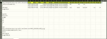
I want to sort this column to rows
Starting from cell A1 every subsequent row be placed in new column B,C,D,E,F,G... till https://..... is encountered


FIND DATA

FORTUNE SOYA BARI 45 G
₹ 9.00
MRP 10.00
Margin ₹1.00
Quantity
Price/Unit
Margin
10+
8.4
1.6
1
Add
FORTUNE SOYA CHUNKS 1 KG
₹ 105.01
MRP 135.00
Margin ₹29.99
Quantity
Price/Unit
Margin
3+
99.01
35.99
1
Add
FORTUNE MINI SOYA 200 G
₹ 36.00
MRP 45.00
Margin ₹9.00
Quantity
Price/Unit
Margin
3+
34
11
1
Add
FORTUNE KGMO JAR 5 L
₹ 695.00
MRP 1,004.00
Margin ₹309.00
Quantity
Price/Unit
Margin
4+
682
322
1
Add
FORTUNE ATTA PP 10 KG
₹ 299.00
MRP 375.00
Margin ₹76.00
Quantity
Price/Unit
Margin
3+
289.91
85.09
1
Add
FORTUNE SOYA CHUNKS 200 G
₹ 36.00
MRP 45.00
Margin ₹9.00
Quantity
Price/Unit
Margin
3+
34
11
1
Add
FORTUNE SOY OIL TIN 15 L
₹ 1,845.00
MRP 2,525.00
Margin ₹680.00
 

Excel Facts

Repeat Last Command
Pressing F4 adds dollar signs when editing a formula. When not editing, F4 repeats last command.
Can you show at least 2-3 rows of how the result should look like? it seems there are empty rows in your single-column data, what happens to those when you transpose?
 
Upvote 0
Can you show at least 2-3 rows of how the result should look like? it seems there are empty rows in your single-column data, what happens to those when you transpose?
Hi,
My bad as it's my first post so do not know right way of conducting things

I have provided new set of Data & it's output
Every Item data starts with image link, starting with https://
Every Item data ends with 1, blank row, Add (all in different rows & these three rows need to be excluded from sorted result)
Blanks rows between data need to be excluded from results


ImageItemRateMRPMarginQuantityPrice/UnitMarginQty Slab 1Rate Slab 1Margin Slab 1Qty Slab 2Rate Slab 2Margin Slab 2
FORTUNE SOYA BARI 45 G FORTUNE SOYA BARI 45 G
9​
MRP 10.00Margin ₹1.00QuantityPrice/UnitMargin10+
8.4​
1.6​
9 FORTUNE SUNFLOWER OIL PP 1 L PK16
2364.8​
MRP 2,960.00Margin ₹595.20QuantityPrice/UnitMargin
MRP 10.00 FORTUNE RB OIL PP 1 L
135.01​
MRP 155.00Margin ₹19.99QuantityPrice/UnitMargin3-11
132.5​
22.5​
12+
131​
24​
Margin ₹1.00
Quantity
Price/Unit
Margin
10+
8.4
1.6
1
Add
FORTUNE SUNFLOWER OIL PP 1 L PK16
2364.8
MRP 2,960.00
Margin ₹595.20
Quantity
Price/Unit
Margin
1
Add
FORTUNE RB OIL PP 1 L
135.01
MRP 155.00
Margin ₹19.99
Quantity
Price/Unit
Margin
3-11
132.5
22.5
12+
131
24
1
Add

Thanks for your time & reply
 

Attachments

  • Transpose Data.png
    Transpose Data.png
    19.5 KB · Views: 12
Upvote 0
Hi Try this! with helper column.

Cell Formulas
RangeFormula
D3:Q6D3=IFERROR(INDEX($A$2:$A$49,MATCH("R"&ROWS($D$3:D3)&"C"&COLUMNS($D$3:D3),$B$2:$B$49,0)),"")
B2:B49B2=IF(OR(A2="",A2=1,A2="Add"),"","R"&SUMPRODUCT(--(LEFT($A$2:A2,6)="https:"))&"C"&COUNTA($A$2:A2)-(COUNTA($A$1:INDEX($A$2:$A$49,AGGREGATE(14,6,(ROW($A$2:A2)-ROW($A$2)+1)/(LEFT($A$2:A2,6)="https:"),1)))-1))
 
Upvote 0
Or with a macro
VBA Code:
Sub escaagrovet()
   Dim Ary As Variant, Nary As Variant
   Dim r As Long, nr As Long, nc As Long
   Dim Cl As Range
   
   Ary = Range("A1", Range("A" & Rows.Count).End(xlUp)).Value
   ReDim Nary(1 To UBound(Ary), 1 To 20)
   
   For r = 1 To UBound(Ary)
      If Left(Ary(r, 1), 6) = "https:" Then
         nr = nr + 1
         nc = 1
         Nary(nr, nc) = Ary(r, 1)
      ElseIf Ary(r, 1) <> "" And Ary(r, 1) <> "Add" And Ary(r, 1) <> 1 Then
         nc = nc + 1
         Nary(nr, nc) = Ary(r, 1)
      End If
   Next r
   Range("C1").Resize(, 14).Value = Array("Image", "Item", "Rate", "MRP", "Margin", "Quantity", "Price/Unit", "Margin", "Qty Slab 1", "Rate Slab 1", "Margin Slab 1", "Qty Slab 2", "Rate Slab 2", "Margin Slab 2")
   Range("C2").Resize(nr, 20).Value = Nary
   For Each Cl In Range("C2").Resize(nr)
      Cl.Hyperlinks.Add Cl, Cl.Value
   Next Cl
End Sub
 
Upvote 0
Sub escaagrovet() Dim Ary As Variant, Nary As Variant Dim r As Long, nr As Long, nc As Long Dim Cl As Range Ary = Range("A1", Range("A" & Rows.Count).End(xlUp)).Value ReDim Nary(1 To UBound(Ary), 1 To 20) For r = 1 To UBound(Ary) If Left(Ary(r, 1), 6) = "https:" Then nr = nr + 1 nc = 1 Nary(nr, nc) = Ary(r, 1) ElseIf Ary(r, 1) <> "" And Ary(r, 1) <> "Add" And Ary(r, 1) <> 1 Then nc = nc + 1 Nary(nr, nc) = Ary(r, 1) End If Next r Range("C1").Resize(, 14).Value = Array("Image", "Item", "Rate", "MRP", "Margin", "Quantity", "Price/Unit", "Margin", "Qty Slab 1", "Rate Slab 1", "Margin Slab 1", "Qty Slab 2", "Rate Slab 2", "Margin Slab 2") Range("C2").Resize(nr, 20).Value = Nary For Each Cl In Range("C2").Resize(nr) Cl.Hyperlinks.Add Cl, Cl.Value Next Cl End Sub
hi,
thanks for helping out.
It is working well with 3 - 4 items but as soon as I increase items, let's say 13-15, it shows error
Runtime Error '9'
Subscript out of range


and if I debug, following line open in yellow highlight
Nary(nr, nc) = Ary(r, 1)

Your help is duly appreciated
 
Upvote 0
Hi Try this! with helper column.

Cell Formulas
RangeFormula
D3:Q6D3=IFERROR(INDEX($A$2:$A$49,MATCH("R"&ROWS($D$3:D3)&"C"&COLUMNS($D$3:D3),$B$2:$B$49,0)),"")
B2:B49B2=IF(OR(A2="",A2=1,A2="Add"),"","R"&SUMPRODUCT(--(LEFT($A$2:A2,6)="https:"))&"C"&COUNTA($A$2:A2)-(COUNTA($A$1:INDEX($A$2:$A$49,AGGREGATE(14,6,(ROW($A$2:A2)-ROW($A$2)+1)/(LEFT($A$2:A2,6)="https:"),1)))-1))
Thanks friend for your work it is working fine.
 
Upvote 0
What is the maximum number of columns you are likely to get?
 
Upvote 0
Hi Try this! with helper column.

Cell Formulas
RangeFormula
D3:Q6D3=IFERROR(INDEX($A$2:$A$49,MATCH("R"&ROWS($D$3:D3)&"C"&COLUMNS($D$3:D3),$B$2:$B$49,0)),"")
B2:B49B2=IF(OR(A2="",A2=1,A2="Add"),"","R"&SUMPRODUCT(--(LEFT($A$2:A2,6)="https:"))&"C"&COUNTA($A$2:A2)-(COUNTA($A$1:INDEX($A$2:$A$49,AGGREGATE(14,6,(ROW($A$2:A2)-ROW($A$2)+1)/(LEFT($A$2:A2,6)="https:"),1)))-1))
A small problem is there
In my system help value is starting from R1C0
So image link is not getting Pasted to columns

Please provide help
 
Upvote 0

Forum statistics

Threads
1,215,563
Messages
6,125,554
Members
449,237
Latest member
Chase S

We've detected that you are using an adblocker.

We have a great community of people providing Excel help here, but the hosting costs are enormous. You can help keep this site running by allowing ads on MrExcel.com.
Allow Ads at MrExcel

Which adblocker are you using?

Disable AdBlock

Follow these easy steps to disable AdBlock

1)Click on the icon in the browser’s toolbar.
2)Click on the icon in the browser’s toolbar.
2)Click on the "Pause on this site" option.
Go back

Disable AdBlock Plus

Follow these easy steps to disable AdBlock Plus

1)Click on the icon in the browser’s toolbar.
2)Click on the toggle to disable it for "mrexcel.com".
Go back

Disable uBlock Origin

Follow these easy steps to disable uBlock Origin

1)Click on the icon in the browser’s toolbar.
2)Click on the "Power" button.
3)Click on the "Refresh" button.
Go back

Disable uBlock

Follow these easy steps to disable uBlock

1)Click on the icon in the browser’s toolbar.
2)Click on the "Power" button.
3)Click on the "Refresh" button.
Go back
Back
Top