Trying to create a snake draft

[thp510]

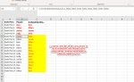
I have a list of 3 individuals that I would like to assign using a snake draft (similar to a fantasy football style draft), where the the last person to pick something is the next person to pick. For example, there are 3 people (Amy, John, Bob) and here's their pick order: Amy goes 1st, John goes 2nd, and Bob goes 3rd. Here's the first 12th pick order.

1st Pick: Amy
2nd Pick: John
3rd Pick: Bob
4th Pick: Bob
5th Pick: John
6th Pick: Amy
7th Pick: Amy
8th Pick: John
9th Pick: Bob
10th Pick: Bob
11th Pick: John
12th Pick: Amy

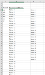
You get the picture. I want to create an equation where I can just populate the first 3 names and then drag the rest of the cells down the rows.

What equation would I put in cell C4?

 

[Fluff]

In what way is it not working?

 

[thp510]

Hi Fluff. Here's a view with my code (pic). It looks like it's just one off and I can't for the life of me figure out why that is.

 

[Fluff]

The first cell the formula goes in should have ROW(A1), not A2

 

[Eric W]

Here's a slightly different approach:

Book1
	A	B	C
1	Pick 1	Amy	Amy
2	Pick 2	John	John
3	Pick 3	Bob	Bob
4	Pick 4	Bob
5	Pick 5	John
6	Pick 6	Amy
7	Pick 7	Amy
8	Pick 8	John
9	Pick 9	Bob
10	Pick 10	Bob
11	Pick 11	John
12	Pick 12	Amy
13	Pick 13	Amy
14	Pick 14	John
15	Pick 15	Bob
16	Pick 16	Bob
17	Pick 17	John
18	Pick 18	Amy
Sheet1

Cell Formulas
Range	Formula
A1:A18	A1	="Pick "&ROW()
B1:B18	B1	=INDEX(C:C,ABS(IF(MOD(ROW()-1,COUNTA(C:C)*2)<COUNTA(C:C),-1,COUNTA(C:C)*2)-MOD(ROW()-1,COUNTA(C:C)*2)))

Put a list of your names in column C. Put the B1 formula in and drag down. If you have more names, just add them to column C and the formula will automatically adjust.

 

[thp510]

The first cell the formula goes in should have ROW(A1), not A2

Amazing! Thank you thank you thank you!

 

[Fluff]

You're welcome, but Eric has a much nicer way of doing it & easier to change the number of people.

 

[thp510]

Here's a slightly different approach:

Book1
	A	B	C
1	Pick 1	Amy	Amy
2	Pick 2	John	John
3	Pick 3	Bob	Bob
4	Pick 4	Bob
5	Pick 5	John
6	Pick 6	Amy
7	Pick 7	Amy
8	Pick 8	John
9	Pick 9	Bob
10	Pick 10	Bob
11	Pick 11	John
12	Pick 12	Amy
13	Pick 13	Amy
14	Pick 14	John
15	Pick 15	Bob
16	Pick 16	Bob
17	Pick 17	John
18	Pick 18	Amy
Sheet1

Cell Formulas
Range	Formula
A1:A18	A1	="Pick "&ROW()
B1:B18	B1	=INDEX(C:C,ABS(IF(MOD(ROW()-1,COUNTA(C:C)*2)<COUNTA(C:C),-1,COUNTA(C:C)*2)-MOD(ROW()-1,COUNTA(C:C)*2)))

Put a list of your names in column C. Put the B1 formula in and drag down. If you have more names, just add them to column C and the formula will automatically adjust.

This is great as well. Thank you so much!

 

[Eric W]

One thought. If you put a heading row, like in your example from post 12, you'd need to change ROW() to ROW(A1) in the first row you put the formula, like in Fluff's case. If you put a heading on the C column where the names are, change COUNTA(C:C) to COUNTA(C$2:C$99) everywhere.

Anyway, I'm glad you got something that works for you!

 

[thp510]

One thought. If you put a heading row, like in your example from post 12, you'd need to change ROW() to ROW(A1) in the first row you put the formula, like in Fluff's case. If you put a heading on the C column where the names are, change COUNTA(C:C) to COUNTA(C$2:C$99) everywhere.

Anyway, I'm glad you got something that works for you!

Hi Eric. Quick follow up question. I did the method you had recommended however my lists starts at at the 4th person down the list versus the 1st person. See pic.

In cell B4 I'm using the formula: =INDEX($D$4:$D$26,ABS(IF(MOD(ROW(A4)-1,COUNTA($D$4:$D$26)*2)<COUNTA($D$4:$D$26),-1,COUNTA($D$4:$D$26)*2)-MOD(ROW(A4)-1,COUNTA($D$4:$D$26)*2)))

Do you know how B4 gives me "Name 1" versus "Name 4"?

Thank you again!

 

[Eric W]

Even though your formula is in B4, you need to put A1 in it, instead of A4. Or this might be a little clearer:

Book1
	A	B	C	D
1
2
3	Account	Recommended Owner
4	aaa	Name 1		Name 1
5	bbb	Name 2		Name 2
6	ccc	Name 3		Name 3
7	ddd	Name 4		Name 4
8	eee	Name 5		Name 5
9	fff	Name 6		Name 6
10		Name 7		Name 7
11		Name 8		Name 8
12		Name 9		Name 9
13		Name 10		Name 10
14		Name 11		Name 11
15		Name 12		Name 12
16		Name 13		Name 13
17		Name 14		Name 14
18		Name 15		Name 15
19		Name 16		Name 16
20		Name 17		Name 17
21		Name 18		Name 18
22		Name 19		Name 19
23		Name 20		Name 20
24		Name 21		Name 21
25		Name 22		Name 22
26		Name 23		Name 23
27		Name 23
28		Name 22
29		Name 21
Sheet25

Cell Formulas
Range	Formula
B4:B29	B4	=INDEX($D$4:$D$99,ABS(IF(MOD(ROWS(B$4:B4)-1,COUNTA($D$4:$D$99)*2)<COUNTA($D$4:$D$99),-1,COUNTA($D$4:$D$99)*2)-MOD(ROWS(B$4:B4)-1,COUNTA($D$4:$D$99)*2)))