Type in field to jump to first instance of what was typed from a drop down list

[ipbr21054]

Hi,
On my worksheet called INV i have a drop down in cell G13
Cell G13 is linked to another worksshet called DATABASE & looks at the customers names in column A

When i create an invoice i use the drop down & then scroll to the customer in question & make the selection.
Once done all my other cells on the INV worksheet get populated with the data on the customers row on the DATABASE sheet.

The above works fine.

Now my list of customers on the worksheet DATABASE is getting longer i am spending longer scrolling through the list of names on INV cell G13
So i need to look at this.

Any suggestions ?
Only one i can think of is if i type T in G13 when i then click the drop down arrown i see the customer selection list start at T as opposed at the begining with A

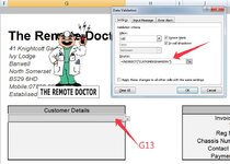
The info for G13 drop down i have found is shown in screenshot

 

[mumps]

Replace the current Worksheet_Change macro in the DATABASE sheet code module with this version:

Private Sub Worksheet_Change(ByVal Target As Range)
    Dim rng As Range, cell As Range, rName As Range, Val As String
    Set rng = Intersect(Target, Range("6:" & Rows.Count), Range("A:Z"))
'   Exit if nothing entered into out target range
    If rng Is Nothing Then Exit Sub
'   Loop through all cells in our target range
    Application.EnableEvents = False
    For Each cell In rng
        UCase (cell.Value2)
    Next cell
    Application.EnableEvents = True
    If Not Intersect(Target, Range("L6:L" & Range("L" & Rows.Count).Row)) Is Nothing And Target.Cells.Count = 1 Then
        Application.EnableEvents = True
        With Target
            .Interior.ColorIndex = 6
            .Font.Size = 11
            .BorderAround xlContinuous, xlThin
            .Font.NAME = "Calibri"
            .Font.Bold = True
            .HorizontalAlignment = xlCenter
            .VerticalAlignment = xlVAlignCenter
        End With
    End If
    Application.ScreenUpdating = False
    Range("P:P").Font.Size = 16
    If Not Intersect(Target, Range("A:A")) Is Nothing Then
        For Each rName In Range("A6", Range("A" & Rows.Count).End(xlUp))
            If rName.Offset(, 15) = "" Then
                If Val = "" Then Val = rName Else Val = Val & "," & rName
            End If
        Next rName
        If Target <> "" Then
            With Sheets("INV").Range("G13").Validation
                .Delete
                .Add Type:=xlValidateList, Formula1:=Val
            End With
        End If
    End If
    Application.ScreenUpdating = True
End Sub

 

[ipbr21054]

Thanks,ive now changed it.

I will monitor it for a day or two to see what happens.

Thanks

 

[ipbr21054]

@mumps
Hi,
Ive have noticed an issue with this change event code on the DATABASE sheet

I use a code which inserts a new row at row 6 & enters a new customers name into cell A6
With you code in use the row gets inserted BUT i then see a RTE13
When i debug the line in your advised code is RED.

MY ORIGINAL CODE

Private Sub Worksheet_Change(ByVal Target As Range)

    Dim rng As Range
    Dim cell As Range
    Set rng = Intersect(Target, Range("6:" & Rows.Count), Range("A:AC"))
   
'   Exit if nothing entered into out target range
    If rng Is Nothing Then Exit Sub
   
'   Loop through all cells in our target range
    Application.EnableEvents = False
    For Each cell In rng
        UCase (cell.Value2)
    Next cell
    Application.EnableEvents = True
   
        If Not Intersect(Target, Range("L6:L" & Range("L" & Rows.Count).Row)) Is Nothing And Target.Cells.Count = 1 Then
   
        Application.EnableEvents = True
       
        With Target
            .Interior.ColorIndex = 6
            .Font.Size = 11
            .BorderAround xlContinuous, xlThin
            .Font.NAME = "Calibri"
            .Font.Bold = True
            .HorizontalAlignment = xlCenter
            .VerticalAlignment = xlVAlignCenter
           
        End With
    
    End If
    Range("P:P").Font.Size = 16
    
  End Sub

YOUR LAST CODE ADVISED

Private Sub Worksheet_Change(ByVal Target As Range)
    Dim rng As Range, cell As Range, rName As Range, Val As String
    Set rng = Intersect(Target, Range("6:" & Rows.Count), Range("A:Z"))
'   Exit if nothing entered into out target range
    If rng Is Nothing Then Exit Sub
'   Loop through all cells in our target range
    Application.EnableEvents = False
    For Each cell In rng
        UCase (cell.Value2)
    Next cell
    Application.EnableEvents = True
    If Not Intersect(Target, Range("L6:L" & Range("L" & Rows.Count).Row)) Is Nothing And Target.Cells.Count = 1 Then
        Application.EnableEvents = True
        With Target
            .Interior.ColorIndex = 6
            .Font.Size = 11
            .BorderAround xlContinuous, xlThin
            .Font.NAME = "Calibri"
            .Font.Bold = True
            .HorizontalAlignment = xlCenter
            .VerticalAlignment = xlVAlignCenter
        End With
    End If
    Application.ScreenUpdating = False
    Range("P:P").Font.Size = 16
    If Not Intersect(Target, Range("A:A")) Is Nothing Then
        For Each rName In Range("A6", Range("A" & Rows.Count).End(xlUp))
            If rName.Offset(, 15) = "" Then
                If Val = "" Then Val = rName Else Val = Val & "," & rName
            End If
        Next rName
        If Target <> "" Then
            With Sheets("INV").Range("G13").Validation
                .Delete
                .Add Type:=xlValidateList, Formula1:=Val
            End With
        End If
    End If
    Application.ScreenUpdating = True
End Sub

 

[mumps]

I’m out of town for a week so I won’t be able to respond until I return home.

 

[ipbr21054]

Ok no problem.
I can continue until you return.

Many thanks.

 

[mumps]

You cannot have more than one Worksheet_Change macro in any workbook. Please upload the most recent version of your file including all the macros you are using and explain in detail what you are trying to do.

 

[ipbr21054]

I believe i did only have the one.
I have now uploaded the for to allow tyou to look at it.

DOWNLOAD HERE

So DATABASE is where my customers are stored.
The INV sheet is where the invoice is completed.
In cell G13 the code should only show thos customer from the DATABASE sheet that doesnt not have an invoice number assigned to them.
The invoice number is in column P

The issue i was having originally was customers were being shown in the dropdown list in cell G13 on INV sheet.

The original worksheet had an edit applied advised by yourself.
When i came to add a new customer on the DATABASE sheet it would error out & when i debug it would mention as above,basically i think no name was in cell G13 on the INV sheet.

I put the original worksheet change back & now that part is fixed but the customers that shouldnt be in the G13 drop down list are sometimes shown.
Not always but definately do appear.
I also sometimes need to click another cell once or twice to lets say refresh the G13 list for it to only show the correct customers of which at present have no invoice number assigned to them.

Thanks

 

[mumps]

Click here to download your file. Give it a try and if you get the same error, describe in detail the steps you performed just before the error appeared.

 

[ipbr21054]

Not sure what edit was made but i open the file, i see the mouse cursor in an animation affect just going round & around for like 20 seconds.

I right click on any of my command buttons & view code but no code is shown for any of them.
Checking the file i uploaded all workwed fine but this new download file does the opposite

If i right click on the sheet DATABASE in code page it shows me error o[peninf DLL

OK so i go to INV sheet but i see TEST 001 002 003 but no 004 so to me its the same

 

[mumps]

I downloaded the file using the link I posted in Post #28 and it worked properly. I couldn't see any of the conditions you described.