Using the COUNT function to reference added lines

[immyjimmy]

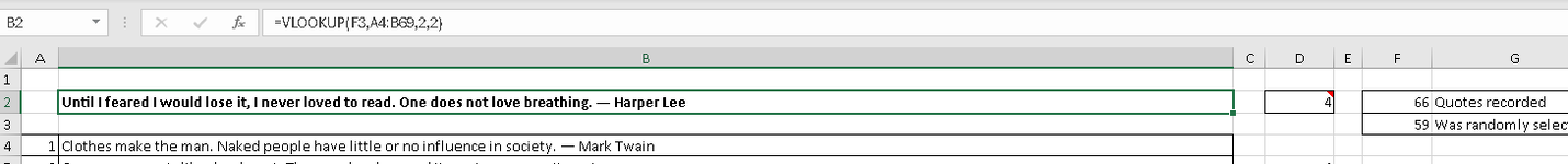
I have a simple workbook that uses a VLOOKUP function.
"=VLOOKUP(F3,A4:B24,2,2)"
As I add data, I have to change the 'B24' to whatever number of rows need to be looked up.
I have another cell (F2) that counts how many rows have data:
"=COUNT(A4:A3000)"
What I'd like to do is have my VLOOKUP function adjust to added lines of data, something like:
=VLOOKUP(F3,A4:B(F2),2,2)
Years ago I remember there being some way of getting the absolute value or referencing or some such, but it's been a long time.
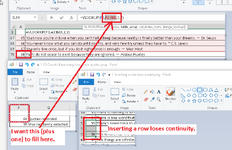
And I know I could name the range, but when I'd add a row in it, I'd have an error in column A with:
=IF(B70="","",A69+1)
Help?

 

[Joe4]

Note that there are easier ways to do it, such as using whole column references in your formula, i.e.
"=VLOOKUP(F3,A:B,2,2)"

Or simply choose a row number that you know you will never exceed, i.e.
"=VLOOKUP(F3,A4:B3000,2,2)"

Also note that if you insert rows into your range, your formula will automatically grow without you having to do anything to do it.
So in your original formula, if you inserted a new row between rows 4:24, this formula:
"=VLOOKUP(F3,A4:B24,2,2)"
will automatically change to this:
"=VLOOKUP(F3,A4:B25,2,2)"

 

[immyjimmy]

Note that there are easier ways to do it, such as using whole column references in your formula, i.e.
"=VLOOKUP(F3,A:B,2,2)"

Or simply choose a row number that you know you will never exceed, i.e.
"=VLOOKUP(F3,A4:B3000,2,2)"

Also note that if you insert rows into your range, your formula will automatically grow without you having to do anything to do it.
So in your original formula, if you inserted a new row between rows 4:24, this formula:
"=VLOOKUP(F3,A4:B24,2,2)"
will automatically change to this:
"=VLOOKUP(F3,A4:B25,2,2)"

I like easy, but it doesn't work here. If I add a quote, my array doesn't grow with it, which is why I'd like the formula to replace the '69' in my VLOOKUP with the value from my COUNT(+1) function in 'F2'. Also, if I insert a row somewhere inbetween, I lose the continuity of the numbers. I want the vaLue of 'F2' to replace the '69' in my VLOOKUP. I'm doing this for someone who's not overly familiar with Excel, and want it to be as easy (I do like easy) as possible.

 

[Joe4]

You have to use the INDIRECT function if you want to build the range dynamically, like this:
=VLOOKUP(F3,INDIRECT("A4:B" & F2),2,2)

By the way, I question what you are doing with the last argument of the function (in red above). "2" isn't really an expected value.
It is expecting a boolean value, i.e. True, False, 0, or 1.
See: Excel VLOOKUP function tutorial with formula examples

 

[immyjimmy]

It was the INDIRECT function I was looking for.
Thanks.

 

[Joe4]

You are welcome.