Using VBA Macro two filter 2 tables on the same sheet

[Excel_User_10k]

Hello "Mr Excel",

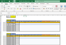
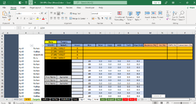
I come to you again for your wisdom haha. I want two tables - One for Targets, and another for Month To Date Sales. Inline with each other as they contain the same structure but separated by a couple of rows. I currently have the following Macro code in place to filter the Target table by the location entered in C6. This is so it only shows the data relevant to that location and so they cannot see each others. I understood the usual rule of "1 filter per sheet" and when I try to copy/paste to create the 2nd table underneath, it causes an issue with the Macro of course. I have uploaded an image of how I would want it to look. Is there away for both of these tables to be filtered at the same time?

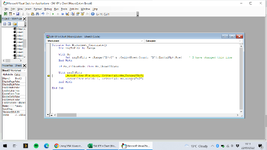
This is the Macro Code I am using:

Private Sub Worksheet_Calculate()

Range(Range("B7"), Range("B7").End(xlDown)).AutoFilter Field:=1, Criteria1:=Range("C6").Value & "*"

End Sub


Hopefully it is an easy solution. Thank You.

 

[Alex Blakenburg]

But the only code I have on this sheet is:

Private Sub Worksheet_Calculate()
Sheets("Targets").Unprotect Password:="password"

Range(Range("B7"), Range("B7").End(xlDown)).AutoFilter Field:=2, Criteria1:=Range("D6").Value & "*"
Range(Range("B7"), Range("B7").End(xlDown)).AutoFilter Field:=1, Criteria1:=Range("E7").Value & "*"

Sheets("Targets").Protect Password:="password"

End Sub

I am using this same code another another Sheet though. Could they be getting in each other's way?

This code is has a couple of errors. Any reason you are not using the code I gave you.
If the code I gave you is not working then tell me what it is not doing.
If it is giving an error message, show me the message and the line of code that is highlighted when you press on the debug button.
If something else is wrong explain what.

 

[Excel_User_10k]

The Help just takes you to this web page, but I imagine that is where you went to download the XL2BB
XL2BB - Excel Range to BBCode

This is unlikely to fix your issue but your With statement in the Reset Sub is not being used and is inconsistent with the rest of the code.
Try and replace it with this:
You are correct as long as those 3 cells are formated as UnLocked, you should not need to unprotect the worksheet for this Sub

Sub Reset_TGT()

    With Sheets("Targets")
        .Unprotect Password:="password"
        .Cells(2, 5) = ""
        .Cells(3, 5) = ""
        .Cells(3, 9) = "Select..."
        .Protect Password:="password"
    End With

End Sub

There was a link at the bottom of this message about it. I take it that will be the same thing. But it isn't working. So forget it. Having enough trouble fixing what I actually need to work haha.

Thank you. That should help that run smoother at least.

It is just this pesky Search Code now, which the whole thing evolves around. Now when I enter the relevant data into the required fields it has some kind of hissy fit and what I think results in a crash. It comes up with the Debug option, and then takes me into the MTD Sheet coding instead when I am on the Targets Sheet. I don't get how that is possible? So this is the code I have on my identical MTD page. Again highlighting one (or the other line) of the Range code. How can they be interfering with each other. Can/should these be edited to be specific to the relevant Sheet as well?

Private Sub Worksheet_Calculate()
Sheets("MTD").Unprotect Password:="stonewall"

With ActiveSheet

Range(Range("B7"), Range("B7").End(xlDown)).AutoFilter Field:=2, Criteria1:=Range("D6").Value & "*"
Range(Range("B7"), Range("B7").End(xlDown)).AutoFilter Field:=1, Criteria1:=Range("E7").Value & "*"

Sheets("MTD").Protect Password:="stonewall"

End With

End Sub

 

[Excel_User_10k]

This code is has a couple of errors. Any reason you are not using the code I gave you.
If the code I gave you is not working then tell me what it is not doing.
If it is giving an error message, show me the message and the line of code that is highlighted when you press on the debug button.
If something else is wrong explain what.

Oh I didn't realise you had sent a second reply. Yes. To use the code you advised, you said I would need to put them into a Table and Name them. I don't think that will fit my purpose.
So 1. I have done something different than having a Target and MTD table auto filter the two underneath each other on one sheet. I have done them on two different Sheets now.
2. I have all 12mths in one solid [unofficial] table with the two hidden columns to filter it all by Store (C) and Month (B).

Perhaps I can give you a better idea with this:

A | B | C | D | E |
April Rochdale Store Store
April Rochdale Employee (FN) Employee (SN)
April Rochdale Employee (FN) Employee (SN)
April Wigan Store Store
April Wigan Employee (FN) Employee (SN)
May Rochdale Store Store
May Rochdale Employee (FN) Employee (SN)
May Wigan Store Store
May Wigan Employee (FN) Employee (SN)


So this continues for the 12mths and all of the employees for each store, all the way down to about row 432. When the store no. and secure id is enters, it shows the Month field. When the month is chosen, it then shows all of the rows like the above but only all of May just for all of Wigan, for instance.

And then on the identical MTD sheet it is the same minus the secure ID. And I have the names entered in Targets to automatically copy over to their MTD equivalent.

Hopefully this paints a clearer picture for you in what I am trying to achieve. If I unhide B and C and manually filter each column then it works perfectly. However, firstly it there is no security this way in that everyone can see everything including each others, and secondly it looks awful for business/professional use. Which is why I am try to use VBA to do it for me instead.

I then created the Reset button because I know that, after entering their own data, they aren't going to bother clearing 3 the fields so it will inevitably be saved with someone's data still showing as it is passed around. Simply being able to click one button after finishing before passing it on is a lot simpler and means they don't need to think about what even needs clearing.

Thank you very much for your patience and for taking the time to continue to help me battle this task of mine.

 

[Alex Blakenburg]

To use the code you advised, you said I would need to put them into a Table and Name them

It does not sound like you have tried the code in post #11. It has nothing to do with having multiple tables it is fixing your code in post #10 (and does the same for your filter post #16).
Come back to me when you have tried it.

 

[Excel_User_10k]

You can give this a try.
Since you seem to have columns B & C filled for all rows I have assumed that when Column D is empty, it indicates the end of the section you want to filter.

As I have mentioned, I am not a fan of using the calculate event for this.
If the change cells are calculations, then perhaps we can trace it back to the underlying cells whose change causes the calculated cells to change.

Private Sub Worksheet_Calculate()
    Dim rngToFltr As Range
   
    With Me
        Set rngToFltr = .Range("B7:C" & .Cells(7, "D").End(xlDown).Row)
    End With
   
    If Me.FilterMode Then Me.ShowAllData
       
    With rngToFltr
        .AutoFilter Field:=2, Criteria1:=Me.Range("D6")
        .AutoFilter Field:=1, Criteria1:=Me.Range("E7")
    End With

End Sub

It does not sound like you have tried the code in post #11. It has nothing to do with having multiple tables it is fixing your code in post #10 (and does the same for your filter post #16).
Come back to me when you have tried it.

OK, fair enough. So I tried it. And it doesn't work. It doesn't filter at all and just comes up with Debug, loads up the code and highlights
.AutoFilter Field:=2, Criteria1:=Me.Range("D6")

Saying Run time error '1004': Autofilter method of Range class failed.


Any ideas?

 

[Alex Blakenburg]

Firsty replace your entire sub by copying in the below ?
(I believe you only have a single table now so I have replaced the xlDown with the xlUp version)

If you then still get an error, turn on the macro recorder and record placing an autofilter on those 3 fields and then post the code it produces using the VBA button here.

Private Sub Worksheet_Calculate()
    Dim rngToFltr As Range
    
    With Me
        Set rngToFltr = .Range("B7:C" & .Cells(Rows.Count, "B").End(xlUp).Row)    ' I have changed this line
    End With
    
    If Me.FilterMode Then Me.ShowAllData
        
    With rngToFltr
        .AutoFilter Field:=2, Criteria1:=Me.Range("D6")
        .AutoFilter Field:=1, Criteria1:=Me.Range("E7")
    End With

End Sub

 

[Excel_User_10k]

Firsty replace your entire sub by copying in the below ?
(I believe you only have a single table now so I have replaced the xlDown with the xlUp version)

If you then still get an error, turn on the macro recorder and record placing an autofilter on those 3 fields and then post the code it produces using the VBA button here.

Private Sub Worksheet_Calculate()
    Dim rngToFltr As Range
   
    With Me
        Set rngToFltr = .Range("B7:C" & .Cells(Rows.Count, "B").End(xlUp).Row)    ' I have changed this line
    End With
   
    If Me.FilterMode Then Me.ShowAllData
       
    With rngToFltr
        .AutoFilter Field:=2, Criteria1:=Me.Range("D6")
        .AutoFilter Field:=1, Criteria1:=Me.Range("E7")
    End With

End Sub

Yeah I have deleted all the code now so it is working ok, just not auto-filtering. Yes just the one table now - which is just a range of cells. I haven't made an official table because they can be a pain to make changes later. That isn't causing an issue is it? Also, I have a few more columns in some rows. But as I am filtering with rows anyway that should be ok shouldn't it?

Ok, I have tried that code. But it is still doing the same thing. It is still this line that it keeps highlighting/having issue with:

.AutoFilter Field:=2, Criteria1:=Me.Range("D6")

With plan B in recording the Macro. How do show that I am trying to have it Filter based on the value of those two Cells in a recording?

 

[Alex Blakenburg]

In the recording just manually select a value for each of the 2 columns you are filtering on.

 

[Excel_User_10k]

Ok, so below is the result of the recording. It only shows the selections I made. How do I edit this to adapt to whatever the Value is in those two Cells? And again to do it dynamically when it is the result of a Formula and not just manually entered? Thank you.

Sub Filter()
'
' Filter Macro
'

'
    Range("D6").Select
    ActiveSheet.Range("$B$7:$C$439").AutoFilter Field:=2, Criteria1:="Bury"
    Range("E7").Select
    ActiveSheet.Range("$B$7:$C$439").AutoFilter Field:=1, Criteria1:="February"
End Sub

 

[Alex Blakenburg]

That all seems consistent with what I have.

I am using the code from post #26 which I can see in your image in # 27 (very helpful) on the sample data below, which you previously provided.
This all works.

The only possibilities would seem to be:
• Is there something noticeably different in your spreadsheet to the data below eg perhaps merged cells ?
• Do you have worksheet protection turned on and if you turn it off does that fix it ?
• Do you have any other Worksheet Events in that sheet module or in the Workbook module ?

If none of that finds the issue, I will need a link to a copy of your workbook.

20220919 VBA Filter Part of Sheet Excel_User_10k v02.xlsm
	A	B	C	D	E	F	G	H	I	J	K	L	M	N	O
1
2				Store No:
3				Secure ID:			Formula
4			Input Value to force calculation ----->			10	20
5
6				Wigan
7				Month	April	Hours	Rev	New	Upgs	HBB	PAYG	Tech	Max	Business	Insurance
8		April	Rochdale	Store	Store	1	25000	4	5	6
9		April	Rochdale	Employee (FN)	Employee (SN)	2		5
10		April	Rochdale	Employee (FN)	Employee (SN)	3		6
11		April	Wigan	Store	Store	4		7
12		April	Wigan	Employee (FN)	Employee (SN)	4		7
13		May	Rochdale	Store	Store
14		May	Rochdale	Employee (FN)	Employee (SN)
15		May	Wigan	Store	Store
16		May	Wigan	Employee (FN)	Employee (SN)
17		March	Bolton	Employee (FN)	Employee (SN)
18		April	Bolton	Employee (FN)	Employee (SN)
19		April	Bolton	Employee (FN)	Employee (SN)
20		April	Halifax	Employee (FN)	Employee (SN)
TestData

Cell Formulas
Range	Formula
G4	G4	=F4+10