Public Sub Collirde_r3()
Const cSourceSheet As String = "Sheet1" ' << Change sheet names as required
Const cDestinationSheet As String = "SUBLIST2"
Dim oWsSrc As Worksheet
Dim oWsDest As Worksheet
Dim rng As Range
Dim arrIN As Variant
Dim arrOUT As Variant
Dim r As Long
Dim n As Long
Dim lRow As Long
Dim iMax As Integer
Dim iBlock As Integer
' unconditionally delete any pre-existing target worksheet
For Each oWsDest In ThisWorkbook.Sheets
If StrComp(cDestinationSheet, oWsDest.Name, vbTextCompare) = 0 Then
Application.DisplayAlerts = False
oWsDest.Delete
Application.DisplayAlerts = True
Exit For
End If
Next
' provide a blank target worksheet
With ThisWorkbook
Set oWsDest = .Sheets.Add(after:=.Sheets(.Sheets.Count))
End With
oWsDest.Name = cDestinationSheet
' allocate memory for source data and perform copy
Set oWsSrc = ThisWorkbook.Sheets(cSourceSheet)
With oWsSrc
' [] this part determines which area within column B has actually been used, starting from cell B3 and downwards
' [] since column B is just one column, Resize statement is used to extend the primary result with some adjacent
' columns at the right hand side, from 1 (col B) to 22 (col W)
' [] the secundary result is a consecutive worksheet area, a matrix with ??? rows and 22 columns
' [] all values of that area are copied into a memory matrix (to increase performance), ie assigned to an array with the name arrIN
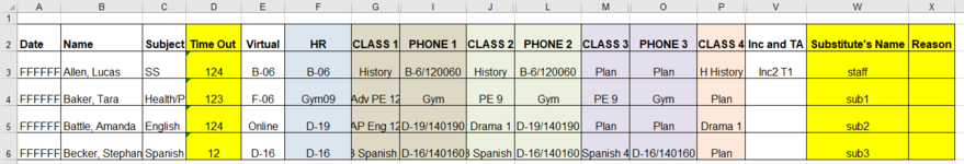
arrIN = .Range("B3", .Cells(.Rows.Count, "B").End(xlUp)).Resize(, 22)
End With
' read source data
For r = 1 To UBound(arrIN, 1) ' [] r represents the "row" number within our memory matrix and is increased by one every turn (Next r)
iMax = Len(arrIN(r, 3)) ' [] "column" 3 (on "row" r) of our matrix contains the "Time Out" numbers without delimiters, so determine how many numbers there are
' allocate memory for destination data
ReDim arrOUT(1 To iMax, 1 To 6) ' [] prepare a memory matrix with iMax rows and 6 columns for the purpose of output on destination sheet
' rearrange destination data
For n = 1 To iMax ' [] on every turn (Next n) fill each row r with the required output
iBlock = Mid(arrIN(r, 3), n, 1) ' [] isolate from row r, column 3 (containing the "Time Out" numbers without delimiters), the required n-th number (length 1) and assign result to iBlock variable
arrOUT(n, 1) = arrIN(r, 1) ' [] copy NAME (column 1) to output matrix (row n, column 1)
arrOUT(n, 2) = iBlock ' [] copy isolated TIME OUT number to output matrix (row n, column 2)
arrOUT(n, 5) = arrIN(r, 21) ' [] copy INC & TA (column 21) to output matrix (row n, column 5)
arrOUT(n, 6) = arrIN(r, 22) ' [] copy SUBSTITUTE'S NAME (column 22) to output matrix (row n, column 6)
Select Case iBlock
Case 1 ' [] depending on TIME OUT number, do copy ....
arrOUT(n, 3) = arrIN(r, 6) ' [] ... row r, column 6 (Class 1) to output matrix
arrOUT(n, 4) = arrIN(r, 7) ' [] ... row r, column 7 (Room 1)
Case 2
arrOUT(n, 3) = arrIN(r, 9) ' [] etc.
arrOUT(n, 4) = arrIN(r, 10)
Case 3
arrOUT(n, 3) = arrIN(r, 12)
arrOUT(n, 4) = arrIN(r, 13)
Case 4
arrOUT(n, 3) = arrIN(r, 15)
arrOUT(n, 4) = arrIN(r, 16)
End Select
Next n
' determine destination area on sheet and paste rearranged data
' [] this part determines the first cell of the area within column A, which area is needed to paste the output to
' [] the resulting cell has to be extended (resized) with a certain number of rows and a certain number of columns so the arrOUT data fits in
' [] the 3 represents worksheet row to start with (row 2 contains headers) and is increased by value lRow on every turn (Next r)
' [] the iMax represents the number of needed rows, the 6 represents the number of needed columns
' [] finally, assign resulting worksheet area to the variable with the name rng
Set rng = oWsDest.Range("A" & 3 + lRow).Resize(iMax, 6)
' [] all values previously placed in memory matrix are pasted into the above determined worksheet area.
rng = arrOUT
' [] adjust target row to start with, with amount of already used rows
lRow = lRow + iMax
Next r
' finally create some headers
With oWsDest.Range("A2:F2")
.Font.Bold = True
.EntireColumn.HorizontalAlignment = xlCenter
.Cells(, 1).EntireColumn.HorizontalAlignment = xlGeneral
' [] within .Cells(row, column) the row number is omitted, so use the only and one row within range ("A2:F2")
.Cells(, 1) = "Teacher Name"
.Cells(, 2) = "Block"
.Cells(, 3) = "Class"
.Cells(, 4) = "Room"
.Cells(, 5) = "Inc and TA"
.Cells(, 6) = "Sub's Name"
End With
rng.EntireColumn.AutoFit
End Sub


 with additional info)