VBA Create a table from two different workbooks based on Active status and report missing data or errors

[Nena99]

I want to merge two tables from two different workbooks and that is what I managed to do so far.
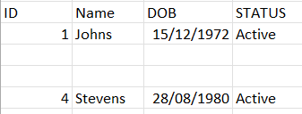
The code I have is good to look for the rows that have active in them but it keeps empty rows in between the new table. Meaning, ID 1 and 4 are active but there is two rows non active and unknown so it wont copy them and I will have similar to the picture
Could someone help me to add a line so it does not leave an empty rows?

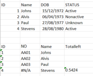
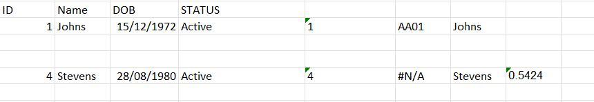
**Also I would like to add a line so it look for the ID in another table and copy the row and bring it to the new table.

**There are errors in the line (4 Stevens) so how can I make it report it back to me that there is error?

Option Explicit

Sub Test()

Dim Cell As Range

With Sheets(1)
   ' loop column H untill last cell with value (not entire column)
   For Each Cell In .Range("G1:G" & .Cells(.Rows.Count, "H").End(xlUp).Row)
       If Cell.Value = "Active" Then
            ' Copy>>Paste in 1-line (no need to use Select)
           .Rows(Cell.Row).Copy Destination:=Sheets(4).Rows(Cell.Row)
           
       End If
   Next Cell
End With

End Sub

 

[Nena99]

file.xlsx
	A	B	C	D	E	F	G	H	I
1	Workbook1
2	ID	Name	DOB	No	DateLeft	STATUS	PostCode
3	1	Johns	15/12/1972	AA000001	15/12/1982	Active	AB1 1AA
4	2	Alvis	06/04/1973	AA000002	06/04/1983	Inactive	AB1 1AA
5	3	Paul	27/08/1977	AA000003	27/08/1987	Unknow	AB1 1AA
6	4	Stevens	28/08/1980	AA000004	28/08/1990	Active	AB1 1AA
7
8	Workbook2
9	ID	NO	Name	Totalleft
10	1	AA01	Johns
11	2	AA02	Alvis
12	3	AA03	Paul
13	4	#N/A	Stevens	0.5424
14
15	New Workbook
16	ID	Name	DOB	No	DateLeft	STATUS	PostCode	Totalleft
17	1	Johns	15/12/1972	AA000001	15/12/1982	Active	AB1 1AA
18	4	Stevens	28/08/1980	AA000004	28/08/1990	Active	AB1 1AA	0.5424
19
20								Total
21
Sheet1

 

[Nena99]

Sorry, it took me a bit of time to figure it out

 

[DacEasy]

Nice, give me an hour, maybe less.

 

[mumps]

Make sure that Workbook1 and Workbook2 are open. Open a new blank workbook and place this macro in a regular module in the new workbook. Also, insert the column headers in row 1 of Sheet1. The macro assumes that the sheet name in each of the 3 workbooks is "Sheet1". In the code change the worksheet names (in red) and the workbook names (in blue) to suit your needs

Sub CreateTable()
    Application.ScreenUpdating = False
    Dim ws1 As Worksheet, ws2 As Worksheet, desWS As Worksheet, fnd As Range, rName As Range
    Set ws1 = Workbooks("Workbook1.xlsx").Sheets("Sheet1")
    Set ws2 = Workbooks("Workbook2.xlsx").Sheets("Sheet1")
    Set desWS = Sheets("Sheet1")
    With ws1
        .Cells(1).CurrentRegion.AutoFilter 6, "Active"
        .AutoFilter.Range.Offset(1).Copy desWS.Cells(desWS.Rows.Count, "A").End(xlUp).Offset(1)
        For Each rName In desWS.Range("B2", desWS.Range("B" & Rows.Count).End(xlUp)).SpecialCells(xlCellTypeVisible)
            Set fnd = ws2.Range("C:C").Find(rName, LookIn:=xlValues, lookat:=xlWhole)
            If Not fnd Is Nothing Then
                rName.Offset(, 6) = fnd.Offset(, 1)
            End If
        Next rName
        .Range("A1").AutoFilter
    End With
    Application.ScreenUpdating = True
End Sub

 

[DacEasy]

Same resluts, but my version :

Option Explicit
Sub forCompareDataOnTwoWorkbooks()

    Dim wbs1 As Workbook: Set wbs1 = Workbooks("mainData.xlsm")
    Dim wbs3 As Workbook: Set wbs3 = Workbooks("transferData.xlsm")
    
    Dim mws1 As Worksheet: Set mws1 = wbs1.Worksheets("Sheet1")
    Dim mws3 As Worksheet: Set mws3 = wbs3.Worksheets("Sheet1")
   
    Dim cell1 As Range, rng1 As Range, lastRow1 As Long
    Dim cell3 As Range, rng3 As Range, lastRow3 As Long
    
    lastRow1 = mws1.Cells(Rows.Count, "B").End(xlUp).Row
    lastRow3 = mws3.Cells(Rows.Count, "C").End(xlUp).Row
    
    Set rng1 = mws1.Range("B2:B" & lastRow1)
    Set rng3 = mws3.Range("C2:C" & lastRow3)

    For Each cell1 In rng1
        For Each cell3 In rng3
        With cell1
            If cell1.Value = cell3.Value Then
            mws1.Range("H" & cell1.Row).Value = mws3.Range("D" & cell3.Row).Value
            
            End If
        End With
        Next cell3
    Next cell1
End Sub

 

[DacEasy]

Set ws1 = Workbooks("Workbook1.xlsx").Sheets("Sheet1")

I will borrow that format for future projects.

 

[Nena99]

Make sure that Workbook1 and Workbook2 are open. Open a new blank workbook and place this macro in a regular module in the new workbook. Also, insert the column headers in row 1 of Sheet1. The macro assumes that the sheet name in each of the 3 workbooks is "Sheet1". In the code change the worksheet names (in red) and the workbook names (in blue) to suit your needs

Sub CreateTable()
    Application.ScreenUpdating = False
    Dim ws1 As Worksheet, ws2 As Worksheet, desWS As Worksheet, fnd As Range, rName As Range
    Set ws1 = Workbooks("Workbook1.xlsx").Sheets("Sheet1")
    Set ws2 = Workbooks("Workbook2.xlsx").Sheets("Sheet1")
    Set desWS = Sheets("Sheet1")
    With ws1
        .Cells(1).CurrentRegion.AutoFilter 6, "Active"
        .AutoFilter.Range.Offset(1).Copy desWS.Cells(desWS.Rows.Count, "A").End(xlUp).Offset(1)
        For Each rName In desWS.Range("B2", desWS.Range("B" & Rows.Count).End(xlUp)).SpecialCells(xlCellTypeVisible)
            Set fnd = ws2.Range("C:C").Find(rName, LookIn:=xlValues, lookat:=xlWhole)
            If Not fnd Is Nothing Then
                rName.Offset(, 6) = fnd.Offset(, 1)
            End If
        Next rName
        .Range("A1").AutoFilter
    End With
    Application.ScreenUpdating = True
End Sub

Thank you but it is not doing anything

 

[Nena99]

Set ws1 = Workbooks("Workbook1.xlsx").Sheets("Sheet1")

I will borrow that format for future projects.

Thank you very much but It should pick the rows based on Active status , I do not want all the rows.
Also, there are missing cells, so it should report there is missing cells.
Can you modify it please?

 

[mumps]

I tested the macro on dummy workbooks using the data you posted and it worked exactly as you requested. Perhaps you could upload copies of your two files to a free site such as www.box.com or www.dropbox.com. Once you do that, mark each file for 'Sharing' and you will be given a link to each file that you can post here (de-sensitized if necessary).

 

[DacEasy]

Ok, this will only pick Active.

Option Explicit
Sub forCompareDataOnTwoWorkbooks()

    Dim wbs1 As Workbook: Set wbs1 = Workbooks("mainData.xlsm")
    Dim wbs3 As Workbook: Set wbs3 = Workbooks("transferData.xlsm")
    
    Dim mws1 As Worksheet: Set mws1 = wbs1.Worksheets("Sheet1")
    Dim mws3 As Worksheet: Set mws3 = wbs3.Worksheets("Sheet1")
   
    Dim cell1 As Range, rng1 As Range, lastRow1 As Long
    Dim cell3 As Range, rng3 As Range, lastRow3 As Long
    
    lastRow1 = mws1.Cells(Rows.Count, "B").End(xlUp).Row
    lastRow3 = mws3.Cells(Rows.Count, "C").End(xlUp).Row
    
    Set rng1 = mws1.Range("B2:B" & lastRow1)
    Set rng3 = mws3.Range("C2:C" & lastRow3)

    For Each cell1 In rng1
        For Each cell3 In rng3
        With cell1
            If cell1.Value = cell3.Value And LCase(mws1.Range("F" & cell1.Row).Value) = LCase("Active") Then
                
                mws1.Range("H" & cell1.Row).Value = mws3.Range("D" & cell3.Row).Value
                
            End If
        End With
        Next cell3
    Next cell1
End Sub