VBA VlookUp not working

[jalrs]

Hello all!

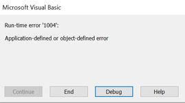
My problem concerns VBA Vlookup. Code simply doesn't work.
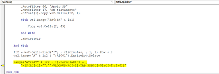
For context: I have two worksheets. One called "Pendentes", the other is called "TAB_FDB". I need to assign a vlookup, so column AY from worksheet "Pendentes" gets autofilled according to column AX picked value. Column AX has a dropdown list where we can pick one value and then we get a value returned on AY(automatically). The matching pair AX->AY, is on the "TAB_FDB" worksheet table. This table is on columns A:B, where A1 and B1 are headers of the table.

My code:

sub myvlookup ()

dim pWS as worksheet, tWS as worksheet
dim pLR as long, tLR as long, x as long
dim datarng as range

set pWS = Thisworkbook.Worksheets("Pendentes")
set tWS = Thisworkbook.Worksheets("TAB_FDB")

pLR = pWS.Range("A" & rows.count).end(xlup).row
tLR = tWS.Range("A" & rows.count).end(xlup).row

set datarng = tWS.Range("A2:B" & tLR)

for x = 2 to pLR

on error resume next
pWS.Range("AY" & x).Value = Application.WorksheetFunction.Vlookup(pWS.Range("AX" & x).Value, datarng, 2, 0)

next x

end sub

any help is greatly appreciated

thanks,
Afonso

 

[jalrs]

The issue is with this line here:

    ws2.UsedRange.Offset(1).ClearContents

It is clearing the entire range of your destination sheet, including the formulas you have in column F!
That is why they are disappearing.

You can use VBA to add those formula back in at the end of your code, like this:

Sub filterApoioSPEXCEL()

    Dim wb1 As Workbook, wb2 As Workbook
    Dim ws1 As Worksheet, ws2 As Worksheet
   
    Set wb1 = ThisWorkbook
    Set wb2 = Workbooks("TemplateExcelVlookUpFormula.xlsm")
   
    Set ws1 = wb1.Worksheets("Stock Trânsito")
    Set ws2 = wb2.Worksheets("Pendentes")
   
    ws2.UsedRange.Offset(1).ClearContents
   
    Dim lr1 As Long, lr2 As Long
   
    lr1 = ws1.Cells(Rows.Count, 1).End(3).Row
    lr2 = ws2.Cells(Rows.Count, 1).End(3).Row + 1
   
    With ws1.Range("A2:D" & lr1)
   
        .AutoFilter 2, "Apoio SP"
        .AutoFilter 3, "Em tratamento"
        .Offset(1).Copy ws2.Cells(lr2, 1)
       
        .AutoFilter
       
    End With
   
    lr2 = ws2.Cells.Find("*", , xlFormulas, , 1, 2).Row + 1
    ws2.Range("A" & lr2 & ":A10").EntireRow.Delete
   
'   Add formulas to column F
    Range("F2:F" & lr2 - 1).FormulaR1C1 = _
        "=IF(RC[-1]="""","""",VLOOKUP(RC[-1],TAB_FDB!C[-5]:C[-4],2,0))"
   
End Sub

Hello Joe,

Do i need to fill any spaces in that line of code? Other than changing range? Because i added that line, changed the range to AY2:AY, and it doesn't seem to be working yet

Thanks

 

[Joe4]

Hello Joe,

Do i need to fill any spaces in that line of code? Other than changing range? Because i added that line, changed the range to AY2:AY, and it doesn't seem to be working yet

Thanks

I went ahead and let your code delete all the formulas, and then just added them back in at the bottom with the section of code entitled "Add formulas to column F".
This should automatically populate the VLOOKUP formulas in column F all the way down to the bottom of your data.

 

[jalrs]

I went ahead and let your code delete all the formulas, and then just added them back in at the bottom with the section of code entitled "Add formulas to column F".
This should automatically populate the VLOOKUP formulas in column F all the way down to the bottom of your data.

Hello Joe,

I noticed that. But when trying to convert it to the proper workbook and not the one I shared with you, i couldn't make it. i came up with this error on attachment

Column of Vlookup is AY. See attachments please

Thanks

 

[Joe4]

You need to make sure that you have adjusted all the row and column references properly to match your file format.

The easiest way to do this is to let Excel figure it out for you!
Turn on your Macro Recorder, and manually create the VLOOKUP formula as it need to appear in one cell in column AY.
Once you have that working the way you need, turn off the Macro Recorder, and view the code you just recorded.
Copy and paste the formula portion of the VLOOKUP formula you created and put it in place of the code we have, specifically the part highlighted in bolded red below:

    Range("AY2:AY" & lr2 - 1).FormulaR1C1 = _
        "=IF(RC[-1]="""","""",VLOOKUP(RC[-1],TAB_FDB!C[-5]:C[-4],2,0))"

 

[jalrs]

You need to make sure that you have adjusted all the row and column references properly to match your file format.

The easiest way to do this is to let Excel figure it out for you!
Turn on your Macro Recorder, and manually create the VLOOKUP formula as it need to appear in one cell in column AY.
Once you have that working the way you need, turn off the Macro Recorder, and view the code you just recorded.
Copy and paste the formula portion of the VLOOKUP formula you created and put it in place of the code we have, specifically the part highlighted in bolded red below:

    Range("AY2:AY" & lr2 - 1).FormulaR1C1 = _
        "=IF(RC[-1]="""","""",VLOOKUP(RC[-1],TAB_FDB!C[-5]:C[-4],2,0))"

Hi Joe,

Range("AY2:AY" & lr2 - 1).FormulaR1C1 = _
        "=IF(RC[-1]="";"";VLOOKUP(RC[-1];TAB_FDB!C[-50]:C[-49];2;0))"

Still get the same error as above.

i went to file -> options -> formula -> reference r1c1 formula and copied and pasted into the highlited bold line of code.

Thanks Joe

 

[Joe4]

What is the value of "lr2" when you get this error?
If you are not sure how to get that, you can just add a MsgBox just before this line of code, i.e.

MsgBox lr2

 

[jalrs]

What is the value of "lr2" when you get this error?
If you are not sure how to get that, you can just add a MsgBox just before this line of code, i.e.

MsgBox lr2

i did that and i got returned the value "2" as attached.

Plus i changed ";" into "," as on your code, but im not getting the values on AY returned after populating AX

 MsgBox lr2
   
    lr2 = ws2.Cells.Find("*", , xlFormulas, , 1, 2).Row + 1
    ws2.Range("A" & lr2 & ":A1001").EntireRow.Delete
   
    Range("AY2:AY" & lr2 - 1).FormulaR1C1 = _
        "=IF(RC[-1]="""","""",VLOOKUP(RC[-1],TAB_FDB!C[-50]:C[-49],2,0))"

Thanks!

 

[Joe4]

OK, that may be your problem.
Why is row 2 shown as the last row?
Shouldn't it go down further?
Is there an issue with that calculation?

 

[jalrs]

OK, that may be your problem.
Why is row 2 shown as the last row?
Shouldn't it go down further?
Is there an issue with that calculation?

Ok so i got help from user @kevin9999 on those lines. He might correct me if i'm wrong:

I think lr2 is related to row1 being the headers. therefore with xlup the macro stops on the last row filled with data after filtering it.
and if no data is found, it clears all the way up until row 2 inclusively. so the headers are safe.

i mean, the template structure is set until row 1000. if it doesnt find data, it clears all rows 2-1000 and leaves the headers. if it finds data in row 30 for example, it clears all the unused template, down from row 31 to row 1000

i hope my explanation makes sense.

Thanks

 

[Joe4]

We can do our own calculation of what row we need to copy down to if you can answer the following:
What column of data will always be populated with data (for any row that has data)?