Very complicated VLOOKUP

[Tricks420]

Hello,

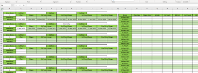
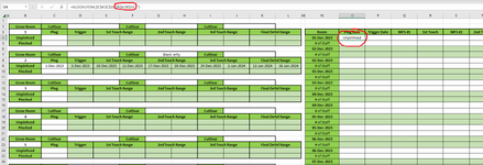
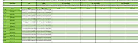
I have a complicated question I have been trying to figure out for hours. I would like a formula for O4 that will look in Column C for the date in N4. Then when it finds it it references the Grow Room number that it was found in, which is located in Column B.

 

[duggie33]

I believe pointing them to a function that would likely work for them is helpful. You do not. We do not have to agree.

 

[Tricks420]

Perhaps something like this:

=XLOOKUP(N4,$C$4:$C$10,$B$4:$B$10,"")

Be sure to adjust the ranges to fit your data.

Hello thank you for your reply however I am getting back "Unpinched" instead of Grow Room 2. Also when I try to extend the ranges I get a #VALUE error.

 

[Tricks420]

I believe pointing them to a function that would likely work for them is helpful. You do not. We do not have to agree.

I've been working on this for hours and don't understand. It is for work and I need an answer ASAP. This is why I am here and asking.

 

[dreid1011]

See if this works for you:

=IFNA(INDEX($B$3:$B$13,MATCH(N4,$C$3:$C$13,0)-IF(XLOOKUP(N4,$C$3:$C$13,$B$3:$B$13,"")="Unpinched",1,2)),"")

 

[Fluff]

Cross-posting (posting the same question in more than one forum) is not against our rules, but the method of doing so is covered by #13 of the Forum Rules.

Be sure to follow & read the link at the end of the rule too!

Cross posted at: Difficult XLOOKUP question
There is no need to repeat the link(s) provided above but if you have posted the question at other places, please provide links to those as well.

If you do cross-post in the future and also provide links, then there shouldn’t be a problem.

 

[6StringJazzer]

I posted this in the cross-posted thread

=LET(M,MATCH(N4,$C:$C,0),INDEX($B:$B,M-IF(INDEX($B:$B,M)="Pinched",2,1)))

 

[6StringJazzer]

I believe pointing them to a function that would likely work for them is helpful. You do not. We do not have to agree.

This needs more than simply switching to XLOOKUP, and if the OP knew how to do it, they wouldn't have needed to ask the question. The problem is "find this row, then move up until you get the number."

 

[Tricks420]

Hey all, it's starting to work the way I need. I changed some of the tables up and it's working. However I am trying to spread the formula to all the required cell in the bottom table. But when I do so it is changing where to look to retrieve the data. I only need the formula on the lines with the dates, not the lines that say "# of Staff". Does anyone know of a quick way? Thank you. Formula is in cell C55 and needs to spreads to C57, C59, C61, etc.

I am trying to upload the file but I can't seem to find the option other then image.

 

[6StringJazzer]

it's starting to work the way I need

There are multiple solutions offered. Which formula are you using?

I am trying to upload the file but I can't seem to find the option other then image.

There is no option to upload a file. You can install the XL2BB add-in (click on the icon in the edit controls). That allows you to select a range, then paste it into a post to show data, formulas, formatting, etc. It's not quite as good as having the file but it's the next best thing.

The question you have in your latest post is quite different than your original question and probably needs a different formula.

 

[Alex Blakenburg]

Formula is in cell C55 and needs to spreads to C57, C59, C61, etc.

Try:

• Select Cells C55:C56 (2 cells)
• Ctrl+C (copy)
• Select an even number of cells to copy 2 eg C57:C68 (multiple of 2)
• Ctrl+V (paste)

If you wanted the formula every 3 rows you would select 3 cells and then your "copy to" range would be a multiple of 3.

Alternatively if you use Jeff's @6StringJazzer formula just change it to ignore the # of Staff rows so that you can copy it to every row but still only get the results on the rows you want it on.

=LET(M,MATCH(N4,$C:$C,0),IF(M4="# of Staff","",INDEX($B:$B,M-IF(INDEX($B:$B,M)="Pinched",2,1))))