VLOOKUP ISSUES

Chris101

New Member
Joined
Feb 17, 2023
Messages
28
Office Version
  1. 365
Platform
  1. Windows
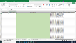
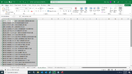
I am trying to use VLOOKUP in VBA. I have a workbook with worksheets "DB Load" and "Service Address". I am looking up "Circuit ID's In sheet "DB Load" (column S) and matching that Circuit ID to the worksheet "service address" where column A contains the Circuit ID's and column B in the worksheet contains the service address', with column B containing the address' that I would like to pull and the fill in column H (Service Address 1) on the DB Load sheet. I hope I did not confuse you.

When I use VLOOKUP manually it works great. but when I try to use my code, well let's just say I get a migraine.

I tried using VLOOKUP two different ways. The first way i used the worksheet function. The second way I tried was copying the formula when I performed the VLOOKUP manually.

Using the worksheet function I get the first 9 rows in column H filled in with the incorrect address but at least I made some progress. A win in my book. The rest of the cells in column H are blank.

Using the method of copying the manual formula I get the first cell filled in but with the correct address. A definite win in my book. however, the rest of the cells are blank.

The two ways that I have tried to write the VLOOKUP are below. If anyone can help me figure out what I am doing wrong would be very much appreciated.

I have also attached a couple of screen shots of the worksheets for review if needed.

Thank you in advance for your time and assistance.

wsh4 is the worksheet "DB Load."
wsh4 is the worksheet "Service Address."


VBA Code:
wsh4.Activate

lastrow = wsh4.Range("A" & Application.Rows.Count).End(xlUp).Row

For j = 2 To lastrow
    wsh4.Range("H" & j).Value = Application.WorksheetFunction.VLookup(wsh4.Range("S2" & j), wsh3.Range("A:B"), 2, 1)
Next j
__________________________________________________________________________________________________________________________________________________
VBA Code:
lastrow = wsh4.Range("A" & Application.Rows.Count).End(xlUp).Row

wsh4.Range("H2").Value = "=VLOOKUP(S2,ServiceAddress,2,TRUE)"

wsh4.Range("H2" & lastrow).FillDown


Thank You,
Chris
 

Attachments

  • DB Load.png
    DB Load.png
    155.2 KB · Views: 6
  • Service Address.png
    Service Address.png
    168.1 KB · Views: 3

Excel Facts

How to calculate loan payments in Excel?
Use the PMT function: =PMT(5%/12,60,-25000) is for a $25,000 loan, 5% annual interest, 60 month loan.
With your second method, try changing TRUE to FALSE in the formula.
 
Upvote 0
With your second method, try changing TRUE to FALSE in the formula.
Peter, I got the same result. One address and the rest of the cells in the column are blank. I really wish I knew what was happening wtih my code.

Thank you very much for your suggestion.
 
Upvote 0
Peter, I got the same result.
In that case can you post some smallish (say 20-30 rows) sample data from each sheet (just columns R:S from 'DB Load' and A:B from 'Service Address') with XL2BB so we can work with a sample of your actual data?
 
Upvote 0
In that case can you post some smallish (say 20-30 rows) sample data from each sheet (just columns R:S from 'DB Load' and A:B from 'Service Address') with XL2BB so we can work with a sample of your actual data?
Yes, of course. I appreciate any help I can get.

Do you mind if I download XL2bBB tomorrow when I get back to the office. It will be around 10pm Est if that's ok.

Thank you very much!

Chris
 
Upvote 0
No problem. :)
As requested sample data for VLOOKUP issue.

The sheet below is the "Service Address" tab showing columns A and B.

BREC.637021..ATI6251 CROOKED CREEK RD NW
BREC.760401..ATI375 RIVERSIDE PKWY
IUEC.707657..ATI3749 WHEELER RD
IZEC.644696..ATI2 EMERSON LN
MLEC.522840..ATI2385 CHAMBLEE TUCKER RD
MLEC.527178..ATI61 FORSYTH ST SW
MLEC.691115..ATI2211 NEW MARKET PKWY SE
MLEC.706951..ATI1 SOUTHWIRE DR
MLEC.729117..ATI6325 PEACHTREE DUNWOODY RD
MLEC.730329..ATI2580 CUMBERLAND PKWY SE
MLEC.781384..ATI75 TED TURNER DR SW
MLEC.793780..ATI1050 TECHWOOD DR NW
MLEC.806862..ATI1074 INDUSTRIAL DR SE
MLEC.826523..ATI1670 CLAIRMONT RD
MLEC.827551..ATI1601 W PEACHTREE ST NE
MLEC.830835..ATI1701 HARDEE AV
MLEC.856289..ATI3003 SUMMIT BLVD
MLEC.857508..ATI1060 TECHWOOD DR NW
MLEC.860743..ATI1700 CLAIRMONT RD
MLEC.871902..ATI4800 BUFORD HWY
MLEC.897688..ATI1295 BARRACKS CT SE
MLEC.910441..ATI3074 CHASTAIN MEADOWS PKW
MLEC.924699..ATI3 SOUTHWIRE DR
MLEC.935828..ATI6305 PEACHTREE DUNWOODY RD
MLEC.941142..ATI6205 PEACHTREE DUNWOODY RD


The below sheet is from the DB Load tab.

Sample Data As Requested for Vlookup.xlsx
HIJKLMNOPQRS
1Service Address 1Service Address 2Service Address 3USOCUSOC DescCRI NotesActive/CanceledCircuit CostHelpdesk Support ChargeBilling Consolidation ChargeSubaccount NoCircuit ID
26251 CROOKED CREEK RD NWBREC.637021..ATI
3BREC.760401..ATI
4IUEC.707657..ATI
5IZEC.644696..ATI
6MLEC.522840..ATI
7MLEC.527178..ATI
8MLEC.691115..ATI
9MLEC.706951..ATI
10MLEC.729117..ATI
11MLEC.730329..ATI
12MLEC.781384..ATI
13MLEC.793780..ATI
14MLEC.806862..ATI
15MLEC.826523..ATI
16MLEC.827551..ATI
17MLEC.830835..ATI
18MLEC.856289..ATI
19MLEC.857508..ATI
20MLEC.860743..ATI
21MLEC.871902..ATI
22MLEC.897688..ATI
23MLEC.910441..ATI
24MLEC.924699..ATI
25MLEC.935828..ATI
DB Load
Cell Formulas
RangeFormula
H2H2=VLOOKUP(S2,ServiceAddress,2,TRUE)


My apologies for being late in downloading the data you requested. When i was downloading XL2BB i kept getting errors.

If you need additional information please let me know.

Thank you for your time and help. it is very much appreciated!

Best Regards,
Chris
 
Upvote 0
Thanks for the sample data. Having that makes it easy to see what was wrong. (I should have seen it anyway, but actual testing is much better than just looking. ;))

Assuming that column A can be used to determine the last row, then just make this change in the last line of the second code posted previously

Rich (BB code):
wsh4.Range("H2:H" & lastrow).FillDown

BTW, instead of entering one formula and using FillDown, you can enter them all at once with this single line of code

VBA Code:
wsh4.Range("H2:H" & lastrow).Formula2 = "=VLOOKUP(S2,ServiceAddress,2,TRUE)"
 
Upvote 0
Solution
Thanks for the sample data. Having that makes it easy to see what was wrong. (I should have seen it anyway, but actual testing is much better than just looking. ;))

Assuming that column A can be used to determine the last row, then just make this change in the last line of the second code posted previously

Rich (BB code):
wsh4.Range("H2:H" & lastrow).FillDown

BTW, instead of entering one formula and using FillDown, you can enter them all at once with this single line of code

VBA Code:
wsh4.Range("H2:H" & lastrow).Formula2 = "=VLOOKUP(S2,ServiceAddress,2,TRUE)"
It is WORKING!!!!!

I really appreciate your help, time and knowledge.

I have about 15 more projects that will require assistance using VBA. When I get stumped can I contact you directly through the board?

I really appreciate your efforts in solving this issue.

Best Regards,
Chris
 
Upvote 0
It is WORKING!!!!!

I really appreciate your help, time and knowledge.

I have about 15 more projects that will require assistance using VBA. When I get stumped can I contact you directly through the board?

I really appreciate your efforts in solving this issue.

Best Regards,
Chris
Both examples work great. And i like the idea of entering the data all at once with one line of code.

Thank You...

Chris
 
Upvote 0

Forum statistics

Threads
1,215,071
Messages
6,122,964
Members
449,094
Latest member
Anshu121

We've detected that you are using an adblocker.

We have a great community of people providing Excel help here, but the hosting costs are enormous. You can help keep this site running by allowing ads on MrExcel.com.
Allow Ads at MrExcel

Which adblocker are you using?

Disable AdBlock

Follow these easy steps to disable AdBlock

1)Click on the icon in the browser’s toolbar.
2)Click on the icon in the browser’s toolbar.
2)Click on the "Pause on this site" option.
Go back

Disable AdBlock Plus

Follow these easy steps to disable AdBlock Plus

1)Click on the icon in the browser’s toolbar.
2)Click on the toggle to disable it for "mrexcel.com".
Go back

Disable uBlock Origin

Follow these easy steps to disable uBlock Origin

1)Click on the icon in the browser’s toolbar.
2)Click on the "Power" button.
3)Click on the "Refresh" button.
Go back

Disable uBlock

Follow these easy steps to disable uBlock

1)Click on the icon in the browser’s toolbar.
2)Click on the "Power" button.
3)Click on the "Refresh" button.
Go back
Back
Top