Xlookup formula to return multiple results

[MissingInAction]

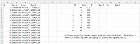
Hi. I have a list of unique IDs (column A) with different dates in column B, C and D. If one of the dates are 1 year old, or older, I want the ID and the age (today() - date in column B, C, D) to be presented in a list in Column I (ID) and Column J (age of date), up to a maximum of 10 results. I currently have an xlookup that does the work for me, but xlookups cant really handle multiple results. I did some Googling and found that Index might help, but I have no knowledge of this formula and online resources aren't very helpful with explaining the Index function.
I have added a screenshot that shows what my formula looks like for cell I2 and J2.

 

[JamesCanale]

The LET functions are worth taking a look at. You can take apart the formula by showing different variables at the end to see how the formula works.

MrExcelPlayground19.xlsx
	A	B	C	D	E	F	G	H	I	J	K	L	M	N
1	ID	Date1	Date2	Date3					ID	Date1	ID	Date2	ID	Date3
2	1	8/12/2023	8/12/2023	8/12/2023				1	3	591	11	848	11	927
3	2	5/12/2023	10/1/2023	6/1/2022				2	7	470	7	546	6	879
4	3	1/1/2022	11/24/2023	9/7/2022				3	6	419			8	832
5	4	8/12/2022	10/9/2023	5/28/2022				4	4	368			7	826
6	5	8/26/2022	6/18/2023	7/7/2022				5					12	818
7	6	6/22/2022	9/10/2023	3/19/2021				6					10	782
8	7	5/2/2022	2/15/2022	5/11/2021				7					9	758
9	8	8/16/2022	5/24/2023	5/5/2021				8					13	685
10	9	10/31/2022	5/4/2023	7/18/2021				9					4	444
11	10	10/8/2022	3/24/2023	6/24/2021				10					2	440
12	11	12/8/2022	4/19/2021	1/30/2021
13	12	3/25/2023	4/3/2023	5/19/2021
14	13	8/4/2023	8/15/2023	9/29/2021
15	14	9/22/2023	12/25/2022	11/25/2022
16	15	9/3/2023	1/1/2023	4/4/2023
Sheet29

Cell Formulas
Range	Formula
I2:J5	I2	=LET(a,A2:A16,b,B2:B16,c,TODAY()-b,d,HSTACK(a,c),dd,FILTER(d,c>365),e,TAKE(SORTBY(d,c,-1),10),f,FILTER(e,TAKE(e,,-1)>364),f)
K2:L3	K2	=LET(a,A2:A16,b,C2:C16,c,TODAY()-b,d,HSTACK(a,c),dd,FILTER(d,c>365),e,TAKE(SORTBY(d,c,-1),10),f,FILTER(e,TAKE(e,,-1)>364),f)
M2:N11	M2	=LET(a,A2:A16,b,D2:D16,c,TODAY()-b,d,HSTACK(a,c),dd,FILTER(d,c>365),e,TAKE(SORTBY(d,c,-1),10),f,FILTER(e,TAKE(e,,-1)>364),f)
Dynamic array formulas.

 

[MissingInAction]

Thank you very much. The more I work with Excel, the more I realize I don't know much about it lol. I'll have to study that formula a while to understand why it works, but for now the important part is, it works.