Year wise calculation

MiyagiSan

New Member
Joined
Mar 23, 2023
Messages
2
Office Version
  1. 365
Platform
  1. Windows
Dear All,

Good Day. I am working at the tuition back office, where I maintain a list of all students, registrations, and their fees. We offer a little discount on fees after the completion of every 12 months.

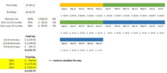
Assume a student began attending classes on August 15, 2022, and continues to do so. After the completion of every 12 months, a discount on the tuition fee will apply for the next 12 months. If a student joins on a certain day in the month, we consider that starting month as a partial month, and we only charge for the number of days of that month. We count 12 months from next month onward unless he joins us on the 1st day of the month. For example, if a student joins on January 10, 2021, then we will count only 21 days, divide the total fee for the month by 21, and start counting 12 months from the February month onwards. If he joins us on January 1, 2021, the counting begins that month. This logic is also the same at the end. The student only has to pay for the number of days he attended in the previous month, not the entire month.


Now I am able to count formulas and calculate Year 1, Year 2, or Year 3, and so on, and see what the total cost is. However, I cannot do the same if I just want to see what he or she paid in 2021. If a student enrolls on July 1, 2021, I will consider the Year 1 total fee until the end of June 2022. However, I am unable to calculate how to detect those dates and calculate the total cost year wise if I want to see what the fee was paid year on year regardless of tuition anniversary and see the breakdown of July 1, 2021, through December 31, 2021, and January 1, 2022, through June 30, 2022. I need your help with this.


I have tried my level best to explain the problem statement. Please see the attached image for better understanding. I apologize for any confusion I have created.

Please guide me.
 

Attachments

  • Tution Fee Calculation - Refer this image.jpg
    Tution Fee Calculation - Refer this image.jpg
    100.7 KB · Views: 16

Excel Facts

Links? Where??
If Excel says you have links but you can't find them, go to Formulas, Name Manager. Look for old links to dead workbooks & delete.
Please post the expectations for the year 2021 months according to the scenario you describe.
 
Upvote 0
Assuming the data are (mis)organized as they are shown in your image, I setup a test sheet as shown belown in the XL2BB minisheet, then calculated in C18 the fee for the year shown in A18 using the formula
Excel Formula:
=LET(Tutto,$F$1:$Q$15,LForY,A18,Inter,TOCOL(Tutto),dDate,FILTER(Inter,IFERROR(YEAR(Inter)>2000,FALSE)),dVal,EXPAND(FILTER(Inter,(IFERROR(YEAR(Inter)<2000,FALSE))*(Inter<>"")),ROWS(dDate),,0),SUMPRODUCT(--(YEAR(dDate)=LForY),dVal))
Copy down for as many headers are in column A

MULTI_C30319.xlsm
ABCDEFGHIJKLMNOPQR
1ago-22set-22ott-22nov-22dic-22gen-23feb-23mar-23apr-23mag-23giu-23lug-23
2
350100100100100100100100100100100100
4
5
6ago-23set-23ott-23nov-23dic-23gen-24feb-24mar-24apr-24mag-24giu-24lug-24
7
8959595959595959595959595
9
10
11ago-24set-24ott-24nov-24dic-24gen-25feb-25mar-25apr-25mag-25giu-25lug-25
12
138585858542,75
14
15
16
17
182022 450,00
192023 1175,00
202024 1047,75
212025 -
Foglio3
Cell Formulas
RangeFormula
G1:Q1,G11:Q11,G6:Q6G1=EDATE(F1,1)
F6,F11F6=EDATE(Q1,1)
C18:C21C18=LET(Tutto,$F$1:$Q$15,LForY,A18,Inter,TOCOL(Tutto),dDate,FILTER(Inter,IFERROR(YEAR(Inter)>2000,FALSE)),dVal,EXPAND(FILTER(Inter,(IFERROR(YEAR(Inter)<2000,FALSE))*(Inter<>"")),ROWS(dDate),,0),SUMPRODUCT(--(YEAR(dDate)=LForY),dVal))
Many thanks for the help and thank you for the time you spent. I have copied the formula and it works. However I have additional question.
Let say, I just enter a price in cell : Like 100 and put start-date, end date - then will it consider discounts and directly give me yearly breakdown like you did over here? I don't wish to add month wise prices manually


2022450
20231175
20241047.75
20250
 
Upvote 0
Are you asking me to put the right data in that (mis)organized structure? No thank you
However I can show a way for putting the data in an ordered list that you can later organize as you prefer

For example, look at the information set in columns A:D of the attached XL2BB minisheet:
-A2 is the enrolling date
-D2 is the standard (starting) fee
-D5 is the yearly discount
-A3 is the next starting date, calculated with the formula =EOMONTH(A2,0)+1
-A3 is copied down to calculate the next starting periods
-B2 is the first monthly Fee, calculated with the formula
Excel Formula:
=LET(EnrollD, $A$2,StartD,A2,MFee,$D$2,YDisc,$D$3,MDays,DAY(EOMONTH(StartD,0)),SDays,MDays-DAY(StartD)+1,YElaps,INT((StartD-EnrollD)/365),cDisc,(1-YDisc)^YElaps,tmFee,MFee*cDisc*SDays/MDays,tmFee)
-Copy B2 down to calculate the next period fee
-After 1 full year the fee will be reduced by the set discount; after a second year a new discount will apply

So that is my basic contribution.

As an additional contribution, consider that you can replicate the calculated information where you prefer, using for example VLOOKUP
For example, see the area G2:T3
-given in row 2 a starting period, for example Jan 2024 in G2
-.. we can import the monthly fee in G3 using the formula =VLOOKUP(G2,$A:$B,2)
-Copy G2 to the next columns to have the next monthly fee

That's all

Cell Formulas
RangeFormula
B2:B31B2=LET(EnrollD, $A$2,StartD,A2,MFee,$D$2,YDisc,$D$3,MDays,DAY(EOMONTH(StartD,0)),SDays,MDays-DAY(StartD)+1,YElaps,INT((StartD-EnrollD)/365),cDisc,(1-YDisc)^YElaps,tmFee,MFee*cDisc*SDays/MDays,tmFee)
H2:T2H2=EOMONTH(G2,0)+1
A3:A31A3=EOMONTH(A2,0)+1
G3:T3G3=VLOOKUP(G2,$A:$B,2)
 
Upvote 0

Forum statistics

Threads
1,215,004
Messages
6,122,659
Members
449,091
Latest member
peppernaut

We've detected that you are using an adblocker.

We have a great community of people providing Excel help here, but the hosting costs are enormous. You can help keep this site running by allowing ads on MrExcel.com.
Allow Ads at MrExcel

Which adblocker are you using?

Disable AdBlock

Follow these easy steps to disable AdBlock

1)Click on the icon in the browser’s toolbar.
2)Click on the icon in the browser’s toolbar.
2)Click on the "Pause on this site" option.
Go back

Disable AdBlock Plus

Follow these easy steps to disable AdBlock Plus

1)Click on the icon in the browser’s toolbar.
2)Click on the toggle to disable it for "mrexcel.com".
Go back

Disable uBlock Origin

Follow these easy steps to disable uBlock Origin

1)Click on the icon in the browser’s toolbar.
2)Click on the "Power" button.
3)Click on the "Refresh" button.
Go back

Disable uBlock

Follow these easy steps to disable uBlock

1)Click on the icon in the browser’s toolbar.
2)Click on the "Power" button.
3)Click on the "Refresh" button.
Go back
Back
Top