A formula to turn a cell red when a date is met

[les361800]

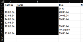
Hello, a simple one I hope (but not for me!)

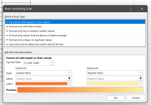
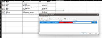
Would anyone mind helping me out with a formula that turns the relevant name cell red when the due date is the following day?
I'm not sure if possible... but is there any way to account for the weekends so if its due on Monday it would turn red on a Friday?

Thank you for any help

 

[Peter_SSs]

If those dates in column C are text (as they appear to be since they are left-aligned) then try this.

24 03 14.xlsm
	B	C
1	Name	Due
2		asap
3		20.03.24
4		20.03.24
5		15.03.24
6
7		15.03.24
8		not urgent
9		15.03.24
Red (2)

Cells with Conditional Formatting
Cell	Condition		Cell Format	Stop If True
B2:B9	Expression	=--SUBSTITUTE(C2,".","/")=WORKDAY(TODAY(),1)	text	NO

If the dates in column C are actual dates but just formatted with dots, then try this

24 03 14.xlsm
	B	C
1	Name	Due
2		asap
3		20.03.24
4		20.03.24
5		15.03.24
6
7		15.03.24
8		not urgent
9		15.03.24
Red

Cells with Conditional Formatting
Cell	Condition		Cell Format	Stop If True
B2:B9	Expression	=C2=WORKDAY(TODAY(),1)	text	NO

 

[les361800]

.

 

[les361800]

If those dates in column C are text (as they appear to be since they are left-aligned) then try this.

24 03 14.xlsm
	B	C
1	Name	Due
2		asap
3		20.03.24
4		20.03.24
5		15.03.24
6
7		15.03.24
8		not urgent
9		15.03.24
Red (2)

Cells with Conditional Formatting
Cell	Condition		Cell Format	Stop If True
B2:B9	Expression	=--SUBSTITUTE(C2,".","/")=WORKDAY(TODAY(),1)	text	NO

If the dates in column C are actual dates but just formatted with dots, then try this

24 03 14.xlsm
	B	C
1	Name	Due
2		asap
3		20.03.24
4		20.03.24
5		15.03.24
6
7		15.03.24
8		not urgent
9		15.03.24
Red

Cells with Conditional Formatting
Cell	Condition		Cell Format	Stop If True
B2:B9	Expression	=C2=WORKDAY(TODAY(),1)	text	NO

Thank you for your reply. I have forgotten how to apply this. Am I in the right function?
I have indeed formatted the column to be dates, but I punched them in with dots.

 

[Peter_SSs]

have forgotten how you apply this.

This is Conditional Formatting
Select from B2 down as far as you might want this to happen, then
Home ribbon tab -> Conditional Formatting -> New rule ... -> Use a formula to determine which cells to format -> Format values where this formula is true:- enter the relevant formula that I gave you -> Format... -> Fill tab -> Choose red -> OK -> OK

 

[Peter_SSs]

I have indeed formatted the column to be dates, but I punched them in with dots.

They still may not be actual dates. Test with a formula like this. If they are actual dates it will return FALSE. Since my example returns TRUE, my date is C2 is not a true date but text.

24 03 14.xlsm
	C	D
3	20.03.24	TRUE
Red (2)

Cell Formulas
Range	Formula
D3	D3	=ISTEXT(C3)

 

[les361800]

They still may not be actual dates. Test with a formula like this. If they are actual dates it will return FALSE. Since my example returns TRUE, my date is C2 is not a true date but text.

24 03 14.xlsm
	C	D
3	20.03.24	TRUE
Red (2)

Cell Formulas
Range	Formula
D3	D3	=ISTEXT(C3)

Thanks, I've changed the dates to have a / between and run that formula - it says true.
The conditional formatting still isnt working though, there's a few names that should be turning red as due tomorrow but nothing is changing

 

[les361800]

They still may not be actual dates. Test with a formula like this. If they are actual dates it will return FALSE. Since my example returns TRUE, my date is C2 is not a true date but text.

24 03 14.xlsm
	C	D
3	20.03.24	TRUE
Red (2)

Cell Formulas
Range	Formula
D3	D3	=ISTEXT(C3)

Another screenshot if helpful...

 

[les361800]

They still may not be actual dates. Test with a formula like this. If they are actual dates it will return FALSE. Since my example returns TRUE, my date is C2 is not a true date but text.

24 03 14.xlsm
	C	D
3	20.03.24	TRUE
Red (2)

Cell Formulas
Range	Formula
D3	D3	=ISTEXT(C3)

Ah wait I was being thick. It's working now, I forgot to change the C to a D as I added a new column!

Thank you very much for your assistance!!
Have a great day Peter

 

[Peter_SSs]

Another screenshot if helpful...

Yes, it shows that you have

1. Not followed my first point "Select from B2 down as far as you might want this to happen". Your image shows the CF is only applied to B2
2. Changed columns
3. Used the formula I suggested for text dates after you have changed the dates to actual (numerical) dates. Use the formula (adjusted for correct column) =C2=WORKDAY(TODAY(),1)