adapt drop down list after selection is made

[robertvdb]

I have the following issue:

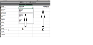
in col A there is a list of cities.
in cell B2, I have a drop down list which contains the values from col A.
in cell C2, I have the value I have selected from the drop down list. In C3, further value after further selection, and so on.

Now, for future selections, I want the drop down list to EXCLUDE the value which is already in C2, C3 and further down.

Any way how to achieve this ? Without VBA ?

 

[awoohaw]

Not really sure if this is what you want. But, this is building drop downs based upon prior lists. I have 365, so I don't get blanks at the bottoms of my drop down list. But, they should only be at the bottom of yours (actually I get one blank).

Book1
	A	B	C	D	E	F	G	H	I	J	K	L	M	N	O	P	Q	R
1	Drop1	Drop2	Drop3	Drop4	Drop5	Drop6	Drop7	Drop8		Drop1	Drop2	Drop3	Drop4	Drop5	Drop6	Drop7	Drop8
2	City2	City1	City11	City5	City6	City3	City9	City7		City1	City1	City3	City3	City3	City3	City4	City4
3										City2	City3	City4	City4	City4	City4	City7	City7
4										City3	City4	City5	City5	City6	City7	City8	City8
5										City4	City5	City6	City6	City7	City8	City9	City10
6										City5	City6	City7	City7	City8	City9	City10
7										City6	City7	City8	City8	City9	City10
8										City7	City8	City9	City9	City10
9										City8	City9	City10	City10
10										City9	City10	City11
11										City10	City11
12										City11
13
14
Sheet4

Cell Formulas
Range	Formula
K2:Q12	K2	=IF(A$2="","",IF((ROW()-1)>(ROWS(J$2:J$12)-1)-(COLUMNS($B$2:$B2)-1),"",INDEX(J$2:J$12,SMALL(IFERROR((ROW(J$2:J$12)-1)/((J$2:J$12<>A$2)),2^1000),ROW()-1))))

Named Ranges
Name	Refers To	Cells
Drop1	=Sheet4!$J$2:$J$12	K2:K12
Drop2	=Sheet4!$K$2:$K$12	L2:L12
Drop3	=Sheet4!$L$2:$L$12	M2:M12
Drop4	=Sheet4!$M$2:$M$12	N2:N12
Drop5	=Sheet4!$N$2:$N$12	O2:O12
Drop6	=Sheet4!$O$2:$O$12	P2:P12
Drop7	=Sheet4!$P$2:$P$12	Q2:Q12

Cells with Data Validation
Cell	Allow	Criteria
A2	List	=Drop1
B2	List	=Drop2
C2	List	=Drop3
D2	List	=Drop4
E2	List	=Drop5
F2	List	=Drop6
G2	List	=Drop7
H2	List	=Drop8

 

[Peter_SSs]

See if this is what you mean. Using a helper column (I have used column F) which could be hidden.
Formula in F2 is copied down to whatever the last row of data is in column A (row 20 in your example)
Use the Data validation shown in the mini sheet for cell B2

24 03 24.xlsm
	A	B	C	D	E	F
1	Cities	Select City	Selected			F2:F9
2	City1		City2			City1
3	City2		City3			City5
4	City3		City4			City6
5	City4		City7			City8
6	City5		City9			City10
7	City6		City12			City11
8	City7		City13			City16
9	City8		City14			City19
10	City9		City15
11	City10		City17
12	City11		City18
13	City12
14	City13
15	City14
16	City15
17	City16
18	City17
19	City18
20	City19
21
DV

Cell Formulas
Range	Formula
F1	F1	=IF(F2="","",ADDRESS(ROW(F2),COLUMN(),4)&":"&ADDRESS(ROW(F2)+COUNTIF(F2:F20,"?*")-1,COLUMN(),4))
F2:F20	F2	=IFERROR(INDEX(A:A,AGGREGATE(15,6,ROW(A$2:A$20)/ISNA(MATCH(A$2:A$20,C:C,0)),ROWS(F$2:F2))),"")

Cells with Data Validation
Cell	Allow	Criteria
B2	List	=INDIRECT(F1)

With the previous selections shown in col C, this is what the DV drop-down now looks like

 

[robertvdb]

Thanks Peter, this seems the right way to work in... Only one question: how do I populate the cells in column C, once I've selected a value in B2 ?

 

[Peter_SSs]

: how do I populate the cells in column C, once I've selected a value in B2 ?

You would have to do that manually or with vba code.
Alternatively, why not have the data validation applied to the cells in column C and the user selects the cities directly in that column?

24 03 24.xlsm
	A	B	C	D	E	F
1	Cities		Selected			F2:F12
2	City1		City5			City2
3	City2		City11			City3
4	City3		City19			City4
5	City4		City10			City7
6	City5		City6			City9
7	City6		City16			City12
8	City7		City1			City13
9	City8		City8			City14
10	City9					City15
11	City10					City17
12	City11					City18
13	City12
14	City13
15	City14
16	City15
17	City16
18	City17
19	City18
20	City19
21
DV (2)

Cell Formulas
Range	Formula
F1	F1	=IF(F2="","",ADDRESS(ROW(F2),COLUMN(),4)&":"&ADDRESS(ROW(F2)+COUNTIF(F2:F20,"?*")-1,COLUMN(),4))
F2:F20	F2	=IFERROR(INDEX(A:A,AGGREGATE(15,6,ROW(A$2:A$20)/ISNA(MATCH(A$2:A$20,C:C,0)),ROWS(F$2:F2))),"")

Cells with Data Validation
Cell	Allow	Criteria
C2:C20	List	=INDIRECT(F$1)

 

[robertvdb]

That's it Peter !

you made my day, Thanks !

 

[robertvdb]

Not really sure if this is what you want. But, this is building drop downs based upon prior lists. I have 365, so I don't get blanks at the bottoms of my drop down list. But, they should only be at the bottom of yours (actually I get one blank).

Book1
	A	B	C	D	E	F	G	H	I	J	K	L	M	N	O	P	Q	R
1	Drop1	Drop2	Drop3	Drop4	Drop5	Drop6	Drop7	Drop8		Drop1	Drop2	Drop3	Drop4	Drop5	Drop6	Drop7	Drop8
2	City2	City1	City11	City5	City6	City3	City9	City7		City1	City1	City3	City3	City3	City3	City4	City4
3										City2	City3	City4	City4	City4	City4	City7	City7
4										City3	City4	City5	City5	City6	City7	City8	City8
5										City4	City5	City6	City6	City7	City8	City9	City10
6										City5	City6	City7	City7	City8	City9	City10
7										City6	City7	City8	City8	City9	City10
8										City7	City8	City9	City9	City10
9										City8	City9	City10	City10
10										City9	City10	City11
11										City10	City11
12										City11
13
14
Sheet4

Cell Formulas
Range	Formula
K2:Q12	K2	=IF(A$2="","",IF((ROW()-1)>(ROWS(J$2:J$12)-1)-(COLUMNS($B$2:$B2)-1),"",INDEX(J$2:J$12,SMALL(IFERROR((ROW(J$2:J$12)-1)/((J$2:J$12<>A$2)),2^1000),ROW()-1))))

Named Ranges
Name	Refers To	Cells
Drop1	=Sheet4!$J$2:$J$12	K2:K12
Drop2	=Sheet4!$K$2:$K$12	L2:L12
Drop3	=Sheet4!$L$2:$L$12	M2:M12
Drop4	=Sheet4!$M$2:$M$12	N2:N12
Drop5	=Sheet4!$N$2:$N$12	O2:O12
Drop6	=Sheet4!$O$2:$O$12	P2:P12
Drop7	=Sheet4!$P$2:$P$12	Q2:Q12

Cells with Data Validation
Cell	Allow	Criteria
A2	List	=Drop1
B2	List	=Drop2
C2	List	=Drop3
D2	List	=Drop4
E2	List	=Drop5
F2	List	=Drop6
G2	List	=Drop7
H2	List	=Drop8

Thanks awoohaw. However, your suggested solution is somewhat complicated, therefore I prefer Peter's solution, see below.

 

[Peter_SSs]

You are welcome. Thanks for the follow-up.