Adding a prefix based on the value of another cell

[sdocherty23]

Hello All,

I need a bit of assistance with adding a prefix to an existing value in a cell based on the value that is in another cell.
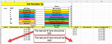
Here is the scenario. I have a field called Job Type. This field has a dropdown list in it that is coming off of a named range in a second sheet in the same workbook.
When I select a value from the Job Type dropdown, such as Residential, it populates the field, but I want to add a prefix of the letter "R" in front of a defined job number in a field called Job #.
An example of this is seen below

The Job # field has a formula in it that I used to generate the job number as seen below:

I am not even sure if it is possible to as an example add the "R" for Residential in front of the -1-23 as a prefix.
Would be very interested in seeing if this is possible.

Thanks

 

[kevin9999]

=IF(F13<>"",XLOOKUP(F13,$C$4:$C$10,$B$4:$B$10,"",0,1)&"-"&ROW()-12&"-23","")

 

[sdocherty23]

=IF(F13<>"",XLOOKUP(F13,$C$4:$C$10,$B$4:$B$10,"",0,1)&"-"&ROW()-12&"-23","")

Thank you very much for this!! It works like a charm.
I have one more question for you about this formula.
In the first image above, I have the left hand job # column (column A) where I want the job numbers to go from 1 - 320
In the second Job # column on the right hand side (column K) I want the job # to go from 321 - 640.
How do I continue the job # in column K

 

[kevin9999]

And presumably the "Job Type" selection for column K would be in column P? If so, then this formula should work in column K:

=IF(P13<>"",XLOOKUP(P13,$C$4:$C$10,$B$4:$B$10,"",0,1)&"-"&ROW()+308&"-23","")

 

[sdocherty23]

Hello kevin9999,

Thank you sooooooo much for your help and very quick reply's!!!
Both of your formula's worked amazing!!

 

[kevin9999]

Hello kevin9999,

Thank you sooooooo much for your help and very quick reply's!!!
Both of your formula's worked amazing!!

You're welcome, and thanks for the feedback

 

[sdocherty23]

You're welcome, and thanks for the feedback

Hello kevin9999,

In regards to the formula that you provided to me, as seen below:
=IF(F13<>"",XLOOKUP(F13,$C$4:$C$10,$B$4:$B$10,"",0,1)&"-"&ROW()-12&"-23","")

The -23 for me is the year. I have a field on the spreadsheet that holds the year as seen below:

Is it possible to have the formula grab the year from the field above highlighted in red and parse out the first two values and add the 23 into the formula so that the year only has to be entered in the Cell beside the word Year and I would not have to change the formula each year?

Let me know if you have any thoughts on this please.

Thank you

 

[kevin9999]

Try this (untested)

=IF(F13<>"",XLOOKUP(F13,$C$4:$C$10,$B$4:$B$10,"",0,1)&"-"&ROW()-12&"-"&Right($B$3,2),"")

 

[sdocherty23]

Try this (untested)

=IF(F13<>"",XLOOKUP(F13,$C$4:$C$10,$B$4:$B$10,"",0,1)&"-"&ROW()-12&"-"&Right($B$3,2),"")

Hello kevin9999,

Once again I have to thank you so very much. The change worked perfectly!