Adding specific word in one cell, results in cells being filled with a certain colour

[MrAlexN]

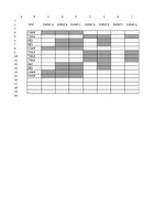
Hope someone can help please. When I type a specific word into column B, I would like the result to show by automatically colouring certain cells in dark grey. For example, if I type BED in cell B16, I would like cells D16, E16, G16 i to fill in dark grey. If I cant have a grey cell, an X will be ok but prefer a colour. Many kind thanks

 

[Micron]

I thought "it can't be too hard to copy and paste a range of interior values because one can copy/paste a range." Google let me down on that. So while it seems a bit more complex than what should be necessary, this does seem to work. If anyone knows how to copy/paste a range of interiors I'm all eyes.

Private Sub Worksheet_Change(ByVal Target As Range)
Dim rng As Range, cel As Range, cel2 As Range
Dim i As Integer, lngColor As Long

If Target.Column = 2 And Target <> "" Then
    With ActiveSheet.Range("B:B")
        Set rng = .Find(Target, LookIn:=xlFormulas)
        If Not rng Is Nothing Then
            For i = 3 To 9
                Set cel = Cells(rng.Row, i)
                Set cel2 = Cells(Target.Row, i)
                lngColor = cel.Interior.Color
                cel2.Interior.Color = lngColor
            Next
        End If
    End With
End If
          
End Sub

 

[MrAlexN]

Hi, I have never created a macro before but happy to try or is this also possible as a formula? If it is not possible to add a cell colour in a formula I’m happy for the cell’s to have an “ X “ in them instead

 

[kevin9999]

Don't be too concerned about macros - you'll learn to love them (isn't that right @Micron )

Right click on the tab name of the sheet where you have your table. Select View Code. Copy the code below & paste it into the window that appears on the right of the screen. Save the file as a macro-enabled workbook and test it. The code is written assuming your "TYPE" column is actually column A (let me know if that's not the case). Whenever you type the name of one of your items in column A, the cells in that row should be filled in grey as per your image.

Private Sub Worksheet_Change(ByVal Target As Range)
    If Target.Cells.CountLarge = 1 And Not Intersect(Range("A:A"), Target) Is Nothing Then
        On Error GoTo Escape
        Dim c As Range, i As Long, a
        Target.Offset(, 1).Resize(, 7).Interior.Color = xlNone
        Select Case UCase(Target.Value2)
            Case Is = "BED"
                a = Array(2, 3, 5)
            Case Is = "CHAIR"
                a = Array(1, 2, 3)
            Case Is = "TABLE"
                a = Array(4, 5, 7)
            Case Else
            GoTo Continue
        End Select
        
        Set c = Target.Offset(, 1).Resize(, 7)
        With c
            .Interior.Color = xlNone
                For i = 0 To UBound(a)
                .Cells(1, a(i)).Interior.Color = RGB(217, 217, 217)
                Next i
        End With
    End If
Continue:
    Application.EnableEvents = True
    Exit Sub
Escape:
    MsgBox "Error " & Err.Number & ": " & Err.Description
    Resume Continue
End Sub

 

[kevin9999]

Got rid of the superfluous clear line:

Private Sub Worksheet_Change(ByVal Target As Range)
    If Target.Cells.CountLarge = 1 And Not Intersect(Range("A:A"), Target) Is Nothing Then
        On Error GoTo Escape
        Dim c As Range, i As Long, a
        Target.Offset(, 1).Resize(, 7).Interior.Color = xlNone
        Select Case UCase(Target.Value2)
            Case Is = "BED"
                a = Array(2, 3, 5)
            Case Is = "CHAIR"
                a = Array(1, 2, 3)
            Case Is = "TABLE"
                a = Array(4, 5, 7)
            Case Else
            GoTo Continue
        End Select
        
        Set c = Target.Offset(, 1).Resize(, 7)
        With c
            For i = 0 To UBound(a)
                .Cells(1, a(i)).Interior.Color = RGB(217, 217, 217)
            Next i
        End With
    End If
Continue:
    Application.EnableEvents = True
    Exit Sub
Escape:
    MsgBox "Error " & Err.Number & ": " & Err.Description
    Resume Continue
End Sub

 

[MrAlexN]

Hi all, thank you for this. I will do as above. My actual “words” are different and the document much bigger and why I needed to automate the process. I’m sure with the template style given above I can substitute in the words I have and also extend this this to work for me. Will be giving it a go later and will update you all. Thank you again

 

[kevin9999]

Hi all, thank you for this. I will do as above. My actual “words” are different and the document much bigger and why I needed to automate the process. I’m sure with the template style given above I can substitute in the words I have and also extend this this to work for me. Will be giving it a go later and will update you all. Thank you again

Glad we could help, and looking forward to hearing how you get on.

 

[MrAlexN]

Hi, sorry, just to check. "C" is the column all these "words" will go in starting at row "4". Then the grey cells will all be in the same row but in different columns

So in my real document I actually type my word "CHAIR" in cell C4, and my cells to have grey boxes are AE4, AX4, BG4, BH4

Do I change the template to:

Case Is = "CHAIR"
a = Array(AE4, AX4, BG4, BH4)

The next line, I add in "BED" in cell C5 and my cells to have grey boxes are AU5, AV5, BC5, BD5

Case Is = "BED"
a = Array(AU5, AV5, BC5, BD5)

is this correct?

Many kind thanks

 

[Micron]

Not because I wrote it, but because it's more flexible. In your real document you can write "fish" if you want and if it's not found, should do nothing. Then you format your cells for fish. Next time you enter fish, it will format that row. Kevin's code will never do anything unless you modify the code to work with "fish", and modify every time you need to add another word to the list. If in your real document you have 50 words you need to deal with, you need 50 Case lines of code. Mine also deals with entries in column B and formats cells 3 to 9, which is what you showed.

 

[MrAlexN]

Hi, would you mind editing your method please just so I can see as I have never done anything like this before and I cant see when I put in what I need

"CHAIR" in cell C4, and my cells to have grey boxes are AE4, AX4, BG4, BH4
"BED" in cell C5 and my cells to have grey boxes are AU5, AV5, BC5, BD5

Private Sub Worksheet_Change(ByVal Target As Range)
Dim rng As Range, cel As Range, cel2 As Range
Dim i As Integer, lngColor As Long

If Target.Column = 2 And Target <> "" Then
With ActiveSheet.Range("B:B")
Set rng = .Find(Target, LookIn:=xlFormulas)
If Not rng Is Nothing Then
For i = 3 To 9
Set cel = Cells(rng.Row, i)
Set cel2 = Cells(Target.Row, i)
lngColor = cel.Interior.Color
cel2.Interior.Color = lngColor
Next
End If
End With
End If

End Sub

Many kind thanks