Array Formula to Remove Zero Value Rows

[Risk]

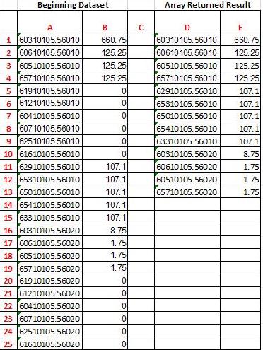
I'm trying to create an array formula to remove zero value rows from a two column dataset, but thus far, I'm only able to accomplish this with a single column dataset which starts in row 1.

{=IF(SUM(IF($B$1:$B$25<>0,1,0))>=ROW(),INDEX($B$1:$B$25,SMALL(IF(($B$1:$B$25)<>0,ROW($B$1:$B$25),""),ROW())),"")}

I'd like to expand this formula to include both columns A & B. Also I think my usage of ROW() is incorrect since if I insert a row above my data set, the array skips my first value "660.75".


Below is what I'm trying to accomplish. Thanks

 

[texasalynn]

try this

Sub RemoveZero()
LR = ActiveSheet.Range("A" & Rows.Count).End(xlUp).Row
'filter data
    Cells.AutoFilter
    Cells.AutoFilter Field:=2, Criteria1:="0"
        Range("B2:B" & LR).EntireRow.Delete
    Cells.AutoFilter
End Sub

 

[Risk]

Thanks for the reply. Sorry I should have mentioned that I wanted to accomplish this without VBA. Plus simply deleting rows ruins a fixed template.

 

[Aladin Akyurek]

I'm trying to create an array formula to remove zero value rows from a two column dataset, but thus far, I'm only able to accomplish this with a single column dataset which starts in row 1.

{=IF(SUM(IF($B$1:$B$25<>0,1,0))>=ROW(),INDEX($B$1:$B$25,SMALL(IF(($B$1:$B$25)<>0,ROW($B$1:$B$25),""),ROW())),"")}

I'd like to expand this formula to include both columns A & B. Also I think my usage of ROW() is incorrect since if I insert a row above my data set, the array skips my first value "660.75".


Below is what I'm trying to accomplish. Thanks

Try...

C1, just enter:

=COUNTIF(B1:B25, ">0")

D1, control+shift+enter, not just enter, copy across, and down:

=IF(ROWS(D$1:D1)<=$C$1,INDEX(A$1:A$25,SMALL(IF($B$1:$B$25>0,
    ROW($B$1:$B$25)-ROW($B$1)+1),ROWS(D$1:D1))),"")

 

[Marcelo Branco]

Maybe this

Select D1 and E1
enter this array-formula
=INDEX($A$1:$B$1000,SMALL(IF($B$1:$B$1000<>0,ROW($B$1:$B$1000)),ROWS($B$1:B1)),0)
Ctrl+Shift+Enter

copy down

HTH

M.

 

[Risk]

Try...

C1, just enter:

=COUNTIF(B1:B25, ">0")

D1, control+shift+enter, not just enter, copy across, and down:

=IF(ROWS(D$1:D1)<=$C$1,INDEX(A$1:A$25,SMALL(IF($B$1:$B$25>0,
    ROW($B$1:$B$25)-ROW($B$1)+1),ROWS(D$1:D1))),"")

Aladin, you never cease to amaze me. Works perfectly. I combined the two step into one

=IF(ROWS(D$1:D1)<=(COUNTIF($B$1:$B$25, ">0")),INDEX(A$1:A$25,SMALL(IF($B$1:$B$25>0,ROW($B$1:$B$25)-ROW($B$1)+1),ROWS(D$1:D1))),"")

This took you all of 10 seconds...you'd laugh if you knew how many hours I'd spent creating my original attempt....

Irony, when I posted this, I had a very strong hunch that you'd be the one to help.

Thanks again

 

[Risk]

Maybe this

Select D1 and E1
enter this array-formula
=INDEX($A$1:$B$1000,SMALL(IF($B$1:$B$1000<>0,ROW($B$1:$B$1000)),ROWS($B$1:B1)),0)
Ctrl+Shift+Enter

copy down

HTH

M.

Thanks Marcelo. I'd need to add another layer to get rid of #NUM!'s, but thank you for helping.

 

[Marcelo Branco]

Thanks Marcelo. I'd need to add another layer to get rid of #NUM!'s, but thank you for helping.

Yes, you are right

Alladin already provided a perfect solution (as usual) but let me try

Select D1:E1
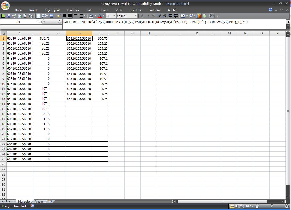
=IFERROR(INDEX($A$1:$B$1000,SMALL(IF($B$1:$B$1000<>0,ROW($B$1:$B$1000)-ROW($B$1)+1),ROWS($B$1:B1)),0),"")
Ctrl+Shift+Enter

copy down

M.

 

[Risk]

Yes, you are right

Alladin already provided a perfect solution (as usual) but let me try

Select D1:E1
=IFERROR(INDEX($A$1:$B$1000,SMALL(IF($B$1:$B$1000<>0,ROW($B$1:$B$1000)-ROW($B$1)+1),ROWS($B$1:B1)),0),"")
Ctrl+Shift+Enter

copy down

M.

Marcelo, you are a gentlemen and a scholar. Thank you for this!

 

[Aladin Akyurek]

Aladin, you never cease to amaze me. Works perfectly. I combined the two step into one

=IF(ROWS(D$1:D1)<=(COUNTIF($B$1:$B$25, ">0")),INDEX(A$1:A$25,SMALL(IF($B$1:$B$25>0,ROW($B$1:$B$25)-ROW($B$1)+1),ROWS(D$1:D1))),"")

This took you all of 10 seconds...you'd laugh if you knew how many hours I'd spent creating my original attempt....

Irony, when I posted this, I had a very strong hunch that you'd be the one to help.

Thanks again

You are welcome. Thanks for providing us feedback.