Array Formula to Remove Zero Value Rows

[Risk]

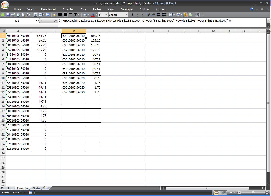
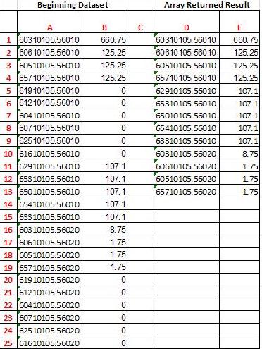
I'm trying to create an array formula to remove zero value rows from a two column dataset, but thus far, I'm only able to accomplish this with a single column dataset which starts in row 1.

{=IF(SUM(IF($B$1:$B$25<>0,1,0))>=ROW(),INDEX($B$1:$B$25,SMALL(IF(($B$1:$B$25)<>0,ROW($B$1:$B$25),""),ROW())),"")}

I'd like to expand this formula to include both columns A & B. Also I think my usage of ROW() is incorrect since if I insert a row above my data set, the array skips my first value "660.75".


Below is what I'm trying to accomplish. Thanks

 

[Marcelo Branco]

Marcelo, you are a gentlemen and a scholar. Thank you for this!

Risk,

Thank you very much for your kind words. I really appreciated!

Tks for the feedback

All the best

M.

 

[nidk27]

Hello,

I have data from cells A1:A76 that I am trying to calculate the most frequent occurrence. The problem I am running into is that the data I have is copied from other sheets and all blank values show up as zero values. I really just need to find the most text occurring in cells A1:A76 and exclude the numbers. Here is the formula I currently have:

=INDEX(A1:A76,MATCH(MAX(COUNTIF($A$1:$A$76,A1:A76)),COUNTIF($A$1:$A$76,A1:A76)))

It is populating 0 as the most frequent occurrence but I want to take those out of the equation and just include the cells that have text.

Any ideas?

Thanks!

 

[Aladin Akyurek]

Hello,

I have data from cells A1:A76 that I am trying to calculate the most frequent occurrence. The problem I am running into is that the data I have is copied from other sheets and all blank values show up as zero values. I really just need to find the most text occurring in cells A1:A76 and exclude the numbers. Here is the formula I currently have:

=INDEX(A1:A76,MATCH(MAX(COUNTIF($A$1:$A$76,A1:A76)),COUNTIF($A$1:$A$76,A1:A76)))

It is populating 0 as the most frequent occurrence but I want to take those out of the equation and just include the cells that have text.

Any ideas?

Thanks!

NAD		1
JAD		2
NAD		MOST FREQ	COUNT
NAD		JAD	4
KAD		VAD	4
VAD
CAD
VAD
XAD
WAD
VAD
JAD
LAD
JAD
VAD
FAD
0
0
QAD
JAD
0
0

<COLGROUP><COL style="WIDTH: 83pt; mso-width-source: userset; mso-width-alt: 3925" width=110><COL style="WIDTH: 21pt; mso-width-source: userset; mso-width-alt: 995" width=28><COL style="WIDTH: 78pt; mso-width-source: userset; mso-width-alt: 3697" width=104><COL style="WIDTH: 58pt; mso-width-source: userset; mso-width-alt: 2759" width=78><TBODY>
</TBODY>

C1: 1 (Adaptable parameter; 1 means the first modus)

C2, control+shift+enter (CSE), not just enter:

=SUM(IF(FREQUENCY(IF($A$2:$A$76<>"",IF(1-ISNUMBER($A$2:$A$76+0),
  MATCH($A$2:$A$76,$A$2:$A$76,0))),ROW($A$2:$A$76)-ROW($A$2)+1)>=
  LARGE(FREQUENCY(IF($A$2:$A$76<>"",MATCH($A$2:$A$76,$A$2:$A$76,0)),
  ROW($A$2:$A$76)-ROW($A$2)+1),C1),1))

This counts in the ties of the first modus if any.

C4, CSE and copy down:

=IF($D4="","",INDEX($A$2:$A$76,SMALL(IF(FREQUENCY(IF($A$2:$A$76<>"",
  IF(1-ISNUMBER($A$2:$A$76+0),MATCH($A$2:$A$76,$A$2:$A$76,0))),
  ROW($A$2:$A$76)-ROW($A$2)+1)=$D4,ROW($A$2:$A$76)-ROW($A$2)+1),
  COUNTIF($D$4:D4,D4))))

D4, CSE and copy down:

=IF(ROWS($D$4:D4)<=$C$2,LARGE(FREQUENCY(IF($A$2:$A$76<>"",
  IF(1-ISNUMBER($A$2:$A$76+0),MATCH($A$2:$A$76,$A$2:$A$76,0))),
  ROW($A$2:$A$76)-ROW($A$2)+1),ROWS($D$4:D4)),"")

 

[KolGuyXcel]

I'm stuck with a similar problem as the original one.

I have "Boolean" data in all the cells in $A$1:$E$200. I'm looking to create a one-dimensional array in column J (or later) where all the cells would have the addresses of the cells in range $A$1:$E$200 which have the value as "TRUE".

 

[Aladin Akyurek]

I'm stuck with a similar problem as the original one.

I have "Boolean" data in all the cells in $A$1:$E$200. I'm looking to create a one-dimensional array in column J (or later) where all the cells would have the addresses of the cells in range $A$1:$E$200 which have the value as "TRUE".

Try to provide a small input sample along with the output which must obtain from that sample.