Assigning Cell Pattern by Reference

[DavidStank]

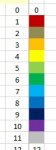
A colleague's spreadsheet uses an IF statement that results in numbers 1-11 and fills the cell with that color (see first attached photo). I don't know how the cell is filled from a single number.
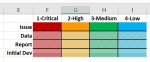
My goal is to find a formula to fill a cell with a pattern based on a reference cell such as those in the second photo. Ideally I would like to have an IF formula with the assignment to fill a cell by reference such as IF(someevaluation, cell format matches format pattern of G3 (as shown in second photo). I have searched the forums but haven't found a way to format a cell's fill pattern based on this kind of reference.
My colleague's options allow for only 11 options for filling where I need 16 with an 'order' to them such as Issue, Data, etc. and whether Critical, High, Medium, or Low priority.
Many thanks in advance for any help.

 

[Yongle]

16 conditional formatting rules can be used to create the colour fills (one rule for each colour)

Is you data laid out in columns ?
which column contains 1-Critical\2-High\3-Medium\4-Low ?
which column contains Issue\Data\Report\Initial Dev ?
which column contains cell to be filled ?

 

[DavidStank]

Hello, Yongle,
The Data is laid out in a single Column where I concatenate 'Type' and 'Severity' like "Issue1-Critical" or "Data3-Medium", etc for tasks on a project as assigned to resources. I fill across a Row like a Gantt chart showing a Resource's workload in hierarchical order: Issue1-Critical / Data1-Critical / Report1-Critical / Initial Dev1-Critical / Issue2-High / Data2-High, etc. etc.
The CellPattern fill I have been able to work uses the formula:
=IF(AND($E21<=I$2,$G21>=I$2),$H21,IF(AND($E22<=I$2,$G22>=I$2),$H22,IF(AND($E23<=I$2,$G23>=I$2),$H23,IF(AND($E24<=I$2,$G24>=I$2),$H24,"")))) for Cell I21 in the photo attached.
Row 21 would show a roll-up task in a Gantt view with the Resource's work displayed in the hierarchy order.

 

[Yongle]

Here is one method using conditional formatting - 16 rules are created (one for each colour)

Sheet "Colours"

Book1
	A	B	C	D	E
1		1-Critical	2-High	3-Medium	4-Low
2	Issue	1	5	9	13
3	Data	2	6	10	14
4	Report	3	7	11	15
5	Initial Dev	4	8	12	16
Colours

"Sheet2" - Result

"Sheet2" - How we get there

cell J2 is date 6 Jan 2020 custom formatted as "DD"
(same for K2,L2 etc)

formula in H3 (copied down)
=INDEX(Colours!$B$2:$E$5,MATCH(C3,Colours!$B$1:$E$1,0),MATCH(D3,Colours!$A$2:$A$5,0))

16 conditional formatting rules are required
select cell J3 when creating each rule
copy J3 down and across

Formula for conditional formatting rule 1
=AND(J$2>=$E3,J$2<=$G3)*$H3=1
and format fill as required

Formula for conditional formatting rule 4
=AND(J$2>=$E3,J$2<=$G3)*$H3=4
and format fill as required

THIS STEP IS NOT REQUIRED BUT IT HELPS EXPLAIN HOW THE SOLUTION WORKS
formula in J3 (copied down and across)
=AND(J$2>=$E3,J$2<=$G3)*$H3
(THE FORMULAS CAN BE DELETED afterwards - the reults in cells are NOT used in the solution)

 

[DavidStank]

Thank you so much. I started down this path but with your suggestions and the formulae I’ll get there much faster.
Again, thank you very much and Happy New Year!