Assigning Values based on a key value

[Knockoutpie]

Hey everyone, for the first time I really have no idea how to go about this..

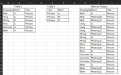
I have a list of people with a title and they all need to be assigned the same document number.

I can see who has what documents, but i'm having issues making a table...

Is there a good way via formula to create a table and have a name repeat for x amount of times based on the number of unique doc#s by title category

the image below shows what i'm trying to achieve, I hope it makes some sense though I understand it's very broad.

I figured maybe there's a combination of formulas I could use, filter, vstack, tocol, etc..

 

[Joe4]

Are you open to a VBA solution?

Also, I am not sure if the "Title" column plays any role here. Will it always be the same for all records for a person?

 

[Knockoutpie]

Are you open to a VBA solution?

Also, I am not sure if the "Title" column plays any role here. Will it always be the same for all records for a person?

of course, i'm open to vba and formula solutions!

The title columns plays a role because I can find all document numbers under a title, once that is done, then I can find what employees with that title do not have a document number, if that makes sense.

 

[rlv01]

The title columns plays a role because I can find all document numbers under a title, once that is done, then I can find what employees with that title do not have a document number, if that makes sense.

I think what @Joe4 is asking, and I have the same question myself, is that if the value of the Title column is always "Person" (presumably a placeholder) for each row of each table as per your example, then it would not seem to play a role in the specific problem you have asked for help with, since all we have to go on is your example.

Btw , when you post an image of your data instead of something that can be copied and pasted into a spreadsheet, it is difficult for others to experiment with it. Which means your chances of getting help drop significantly. Instead, use the free XL2BB tool (link below) to post your data in a way that makes it accessible to others.

XL2BB - Excel Range to BBCode

Excel 'mini-sheet' in messages - XL2BB Although experts prefer to read your description and question instead of working in your actual file to solve your problem, there are times that it is difficult to explain an issue without providing actual...

www.mrexcel.com

 

[Joe4]

OK, here is the VBA code that I came up with:

Sub CreateOutput()

    Dim lr1 As Long, lr2 As Long
    Dim n2 As Long
    Dim r As Long
    Dim i As Long, j As Long
    Dim rng As Range

    Application.ScreenUpdating = False

'   Add titles
    Range("I1") = "Desired Output"
    Range("A2:C2").Copy Range("H2")
    
'   Find last rows of Tables 1 and 2 and count number of records in second table
    lr1 = Cells(Rows.Count, "A").End(xlUp).Row
    lr2 = Cells(Rows.Count, "F").End(xlUp).Row
    n2 = lr2 - 2
    
'   Set initial row number for output table
    r = 3
    
'   Loop through Table1 and populate rows in output table
    For i = 3 To lr1
'       Populates column H and J
        Range(Cells(r, "H"), Cells(r + n2 - 1, "H")) = Cells(i, "A")
        Range(Cells(r, "J"), Cells(r + n2 - 1, "J")) = Cells(i, "C")
'       Loop through table 2 records and populate column I
        For j = 3 To lr2
            Cells(r + j - 3, "I").Formula = "=IF(COUNTIFS($A$3:$A$" & lr1 & ",$H" & r + j - 3 & ",$B$3:$B$" & lr1 & ",$F" & j & ")>0,F" & j & ",""Missing "" & F" & j & ")"
        Next j
'       Increase next row number
        r = r + n2
    Next i
    
'   Autosize output range
    Columns("H:J").EntireColumn.AutoFit

'   Build range to format
    Set rng = Range("H2:J" & r - 1)
    
'   Format range to show grid lines
    With rng.Borders(xlEdgeLeft)
        .LineStyle = xlContinuous
        .ColorIndex = xlAutomatic
        .TintAndShade = 0
        .Weight = xlThin
    End With
    With rng.Borders(xlEdgeTop)
        .LineStyle = xlContinuous
        .ColorIndex = xlAutomatic
        .TintAndShade = 0
        .Weight = xlThin
    End With
    With rng.Borders(xlEdgeBottom)
        .LineStyle = xlContinuous
        .ColorIndex = xlAutomatic
        .TintAndShade = 0
        .Weight = xlThin
    End With
    With rng.Borders(xlEdgeRight)
        .LineStyle = xlContinuous
        .ColorIndex = xlAutomatic
        .TintAndShade = 0
        .Weight = xlThin
    End With
    With rng.Borders(xlInsideVertical)
        .LineStyle = xlContinuous
        .ColorIndex = xlAutomatic
        .TintAndShade = 0
        .Weight = xlThin
    End With
    With rng.Borders(xlInsideHorizontal)
        .LineStyle = xlContinuous
        .ColorIndex = xlAutomatic
        .TintAndShade = 0
        .Weight = xlThin
    End With
    
    Application.ScreenUpdating = True
    
End Sub

And here is the image - I started with "Table 1" and "Table 2" and the VBA code created everything in red.