Auto Highlight Cells

[exelified]

Thanks in Advance:

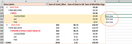
The objective: Identify each mobile device user (and device) who hasn't used their device (at all) - i.e. no voice min. used and no data used over the past three consecutive months (as defined). Note: This is a monthly report so actual months change.

My column E will contain three consecutive instances of the returned value "Zero Use", sporadically, and as a result of conditions met in the formula below. Ex:

ROW COL E
281 Zero Use
282 Zero Use
283 Zero Use

The Question: In a script, how might I go about finding:

1) each 3 consecutively returned value instances of the term "Zero Use" and
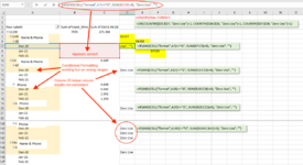
2 then, once found - automatically highlight (relatively) the 3r x 4c just to the left of each instance (or in the case shown with E281) as shown in the attached image

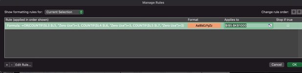
=IF(AND(OR(A281="<12/23/2020",A281="Jan",A281="Feb"),AND(B281=0,C281=0)),"Zero Use","")=IF(AND(OR(A281="<12/23/2020",A281="Jan",A281="Feb"),AND(B281=0,C281=0)),"Zero Use","")

Note:: Formula is set for specific months but I'm thinking that doesn't have to be the case. i.e. any past tree consecutive months will satisfy the requirement.

 

[Roybzer]

I'm not exactly sure how you would go about this in a script, but it would certainly be easy enough to accomplish with conditional formatting:

Condition: =COUNTA($E1:$E5)=3
Range: =$A$3:$D$10000

 

[exelified]

I'm not exactly sure how you would go about this in a script, but it would certainly be easy enough to accomplish with conditional formatting:

Condition: =COUNTA($E1:$E5)=3
Range: =$A$3:$D$10000

Thanks and my apologies but I'm not understanding your solution. What I can gather: The condition, as you're stating, is to count all instances of cells containing anything three times in Column E within an absolute reference range of $E1:$E5 (?) - and to apply that, somehow, throughout the likely range for the table as a conditional format? Could you possibly screen shot the conditional statement in place using the test document I posted here?

 

[Fluff]

Welcome to the MrExcel Message Board!

Cross-posting (posting the same question in more than one forum) is not against our rules, but the method of doing so is covered by #13 of the Forum Rules.

Be sure to follow & read the link at the end of the rule too!

If you have posted the question at more places, please provide links to those as well.

If you do cross-post in the future and also provide links, then there shouldn’t be a problem.

 

[Roybzer]

Thanks and my apologies but I'm not understanding your solution. What I can gather: The condition, as you're stating, is to count all instances of cells containing anything three times in Column E within an absolute reference range of $E1:$E5 (?) - and to apply that, somehow, throughout the likely range for the table as a conditional format? Could you possibly screen shot the conditional statement in place using the test document I posted here?

I only have access to my phone at the moment, but I can send a screenshot tomorrow.

Because there is potential overlap with the proximity of the data, it would just need to be adjusted slightly to ensure consecutive zero use.

Covering the cases in the conditional formula would work:

=OR(COUNTA($E1:$E3)=3, COUNTA($E2:$E4)=3, COUNTA($E3:$E5)=3)

Only the column is absolute, so that when it checks against the range $A$3:$D$1000(or whatever the size of the range) it applies the conditional formatting across A:D based upon column E.

 

[exelified]

I only have access to my phone at the moment, but I can send a screenshot tomorrow.

Because there is potential overlap with the proximity of the data, it would just need to be adjusted slightly to ensure consecutive zero use.

Covering the cases in the conditional formula would work:

=OR(COUNTA($E1:$E3)=3, COUNTA($E2:$E4)=3, COUNTA($E3:$E5)=3)

Only the column is absolute, so that when it checks against the range $A$3:$D$1000(or whatever the size of the range) it applies the conditional formatting across A:D based upon column E.

Ahhh... Clearer thank you!

 

[Roybzer]

Having had a look at the spreadsheet, I think it would be easier if you evaluated L to show 'Zero Use' for each month, then use conditional formatting to check for 3 consecutive instances of 'Zero Use'. This is what the below would achieve:

CONDITION: =OR(COUNTIF($L3:$L5, "Zero Use")=3, COUNTIF($L4:$L6, "Zero Use")=3, COUNTIF($L5:$L7, "Zero Use")=3)
RANGE: $I$5:$K$10000

You would want to avoid the current way of calculating 'Zero Use' on the test spreadsheet as it is not suitable for other other ranges of months given the specification of Jan, Feb and Dec in the formula. Also, the date format on the pivot table should include the year to ensure that the months are consecutive, as they are currently listed as Jan, Feb, Dec.

You can change the date format from the 'Pivot Table Analyse' tab using 'Group Selection' and ungroup(make sure to have selected one of the months on the pivot table before going through this step).

You can then change the format of the date using the field settings to include the month and year.

Once the field format has been changed, you can evaluate 'Zero Use' in column 'L' using:

=IF(AND(CELL("format", I5)<>"G", SUM(J5:K5)=0), "Zero Use", "")

Given that I'm not sure which date format you'll end up using, the above just checks that the format type is not general(the format of the headings), then checks if the minutes and data are zero.

I hope this is of use.

 

[exelified]

Having had a look at the spreadsheet, I think it would be easier if you evaluated L to show 'Zero Use' for each month, then use conditional formatting to check for 3 consecutive instances of 'Zero Use'. This is what the below would achieve:

CONDITION: =OR(COUNTIF($L3:$L5, "Zero Use")=3, COUNTIF($L4:$L6, "Zero Use")=3, COUNTIF($L5:$L7, "Zero Use")=3)
RANGE: $I$5:$K$10000

You would want to avoid the current way of calculating 'Zero Use' on the test spreadsheet as it is not suitable for other other ranges of months given the specification of Jan, Feb and Dec in the formula. Also, the date format on the pivot table should include the year to ensure that the months are consecutive, as they are currently listed as Jan, Feb, Dec.

You can change the date format from the 'Pivot Table Analyse' tab using 'Group Selection' and ungroup(make sure to have selected one of the months on the pivot table before going through this step).

You can then change the format of the date using the field settings to include the month and year.

Once the field format has been changed, you can evaluate 'Zero Use' in column 'L' using:

=IF(AND(CELL("format", I5)<>"G", SUM(J5:K5)=0), "Zero Use", "")

Given that I'm not sure which date format you'll end up using, the above just checks that the format type is not general(the format of the headings), then checks if the minutes and data are zero.

I hope this is of use.

Major ?? are not enough but THANKS for taking the time and for offering what appears to be a very elegant and appropriate solution. I will have a look shortly.

 

[exelified]

Major ?? are not enough but THANKS for taking the time and for offering what appears to be a very elegant and appropriate solution. I will have a look shortly.

Circling back around to update Roybzer: Thanks again. Strangely, you managed to get this to work but so far for me, results have been mixed - even using the same example sheet I provided. A screen shot of the "real world" sheet is attached. Can you tell where I've gone astray of your example?

 

[Roybzer]

Circling back around to update Roybzer: Thanks again. Strangely, you managed to get this to work but so far for me, results have been mixed - even using the same example sheet I provided. A screen shot of the "real world" sheet is attached. Can you tell where I've gone astray of your example?

No worries. Not sure where the discrepancies are, but I'll have a look.

Can you confirm the range that you're using for the conditional format? I see that the screenshot if from row 5, but the original condition was setup from row 3. Range should therefore be $I$7:$K$10000.

I'll have a look at the 'zero use' formula and get back to you.