Auto populate individual cells based off cell values from data table with NO VBA

[Stomli]

Hi Forum,

This is my first time posting. I am usually able to find my answer to other questions by looking through the forums but I haven't been able to find an answer for this issue I'm having. So I am reaching out to the experts on here. Please and Thank you!

I need to auto populate dates for specific users based on cell values inside a table. I would like to implement them with dynamic array formulas so this can scale and update based on new reports. Also, I can't do this with macros or VBA since the end users can't work with them.

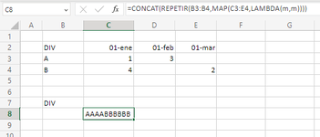
First thing I would need to know is how I would go about is how to make duplicate cells based on values (numbers) in a cell. I have been looking up some nested If functions, but I am not sure how they could work for a multiple month table with blanks in them.

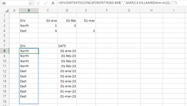
The other thing I need is a method on how to tie these duplicate cells to a unique user I.d. while omitting blank fields for months without changes. I was thinking after the duplication if figured out that a sequence formula could just drag the duplicated dates down and use a filter() formula to match them to the right division.

I could develop the back end in a helper column/tab. If this is too difficult for one direct solution, please suggest methods or formulas that I could use to solve this.

Thanks for your time.

S

 

[DanteAmor]

Hello @Stomli .

Welcome to the MrExcel forum. Please accept my warmest greetings and sincere hope that all is well.


Try the following formulas.

In cell B8:

=MID(CONCAT(REPT(B3:B4,MAP(C3:N4,LAMBDA(m,m)))),SEQUENCE(SUM(C3:N4)),1)

In cell D8:

=LET(a,C3:N4,--MID(CONCAT(REPT(C2:N2,MAP(a,LAMBDA(m,m)))),5*(SEQUENCE(SUM(a))-1)+1,5))

I attached the images so you can see the result.

--------------
Let me know the result and I'll get back to you as soon as I can.
Cordially
Dante Amor
--------------​

 

[DanteAmor]

Also, I noticed the Mid was based off of one character. What would I need to look into for a 3 character division name?

But all must be 3 characters.

=LET(a,C3:N4,MED(CONCAT(REPETIR(B3:B4,MAP(a,LAMBDA(m,m)))),3*(SECUENCIA(SUMA(a))-1)+1,3))

---- *** ----​

Since the dates are going to be tied to the user ID, is there a way to ensure that the user ID corresponds to the date and the division (the division is a lookup based on the user ID)?

You should show me how those IDs are.
The formula obtains the data of the dates and the divisions from left to right and from top to bottom.

---- *** ----​

Could you provide a brief breakdown of how these 2 formulas particularly how the Mid, Concat, Rept, and Sequence tie into each other?

Of course.
If with the formulas before MS365 there were several solutions to the same problem, now with the new MS365 formulas, the number of solutions for the same problem has increased considerably.

I explain my solution, maybe there are more solutions, maybe simpler or more complicated, but this is how I tried to solve it.

I have to tell you that I have barely 2 months of using a version of 365 that is in the cloud and the functions come in English and Spanish, add that it is a slightly different Spanish from the one I usually use in the functions. In fact it is the first time that I use the LAMBDA and MAP functions.

---- *** ----​

how the Mid, Concat, Rept, and Sequence tie into each other?

I will explain using an example of 3 months:

In this case, with the MAP function, I am passing the matrix from C3 to E4 to the LAMBDA function, which in this case does not require doing anything to the matrix, I only need it to return the matrix but applying to each data in the matrix the REPT function:

So in the example cell C3 has a 1, it means that the data in cell B3 is going to be repeated 1 time.
Cell D3 has a 3, it means that the data in cell B3 is going to be repeated 3 times.
Look in the following image how the division is repeated the number of times it appears in the matrix.

The CONCAT function concatenates all the results on a single line. This is the option I found. Maybe there is another solution.

Now the difficult thing is to separate each division in a cell vertically.

To separate the string into rows I use the MID function, this function needs the initial position, for that I use the sequence function, which will give us position 1, 2, 3 and even the total number of characters in the string, how many are? the sum of the numbers in the range C3:E4; and the last parameter of the MID function is the number of characters to take from the string, in this case the division is 1.

​

---- *** ----


I hope the explanation helps you.
Cordially
Dante Amor
--------------​

​

 

[kweaver]

I don't understand your 2nd request. How about this for the first?

062023 Misc.xlsm
	B	C	D	E	F	G	H	I	J	K	L	M	N
2	Div	Jan	Feb	Mar	Apr	May	Jun	Jul	Aug	Sep	Oct	Nov	Dec
3	A	0	2	0	0	1	0	1	0	0	4	0	0
4	B	0	0	0	3	0	0	0	2	0	0	0	0
DateChg

Cell Formulas
Range	Formula
C3:N4	C3	=SUM((--($B$8:$B$20=$B3))*(--MONTH($D$8:$D$20)=COLUMN()-2))

 

[lrobbo314]

kweaver, I think the portion you gave formulas for is being hard coded in. I think Stomli wants to generate the table below with the table above. I've already tried and reverted to PowerQuery to at least get something that works.

But I'm sure they want a formula do generate at least the date column, but probably the division column as well. Haven't been able to get a formula to work yet.

 

[Stomli]

Thanks for your explanation Irobbo314. Yes, that is what I want for the dates column the division is a xlookup that already links the IDs So I don't need any help on that column but I need to get the dates to follow downward from the top of the user id. So I need 2 Feb dates for the 1st 2 users then a May date for the next user. I would need to input these 1 after the other taking into account the months that don't have any dates in them and also the division for each user Id.

 

[Stomli]

Also sorry for the screenshot. My company has my excel locked down so I can't get the add-in.

 

[kweaver]

With several helpers, this does it, I think...but it's a little more effort than really desired.
I haven't figured out a LET function for it or another shorter way.

This might temporarily get you over a hump if there's not too much to handle.

062023 Misc.xlsm
	B	C	D	E	F	G	H	I	J	K	L	M	N
1		1	2	3	4	5	6	7	8	9	10	11	12
2	Div	Jan	Feb	Mar	Apr	May	Jun	Jul	Aug	Sep	Oct	Nov	Dec
3	A	0	2	0	0	1	0	1	0	0	4	0	0
4	B	0	0	0	3	0	0	0	2	0	0	0	0
5
6
7	Div	User	Date		A				B
8	A		2/1/2024		2	2	1	2	3	4	1	4
9	A		2/1/2024		1	5	3	2	2	8	4	4
10	A		5/1/2024		1	7	4	5			6	4
11	A		7/1/2024		4	10	5	7				8
12	A		10/1/2024				9	10				8
13	A		10/1/2024					10
14	A		10/1/2024					10
15	A		10/1/2024					10
16	B		4/1/2024
17	B		4/1/2024
18	B		4/1/2024
19	B		8/1/2024
20	B		8/1/2024
DateChg

Cell Formulas
Range	Formula
C1:N1	C1	=SEQUENCE(,12)
D8:D15	D8	=DATE(2024,I8#,1)
F8:F11	F8	=TRANSPOSE(FILTER(C3:N3,C3:N3<>0))
G8:G11	G8	=TRANSPOSE(FILTER(C1#,$C$3:$N$3<>0))
I8:I15	I8	=XLOOKUP(SEQUENCE(SUM(F8#)),H8:H12,G8:G12,,-1)
J8:J9	J8	=TRANSPOSE(FILTER(C4:N4,C4:N4<>0))
K8:K9	K8	=TRANSPOSE(FILTER(C1#,$C$4:$N$4<>0))
M8:M12	M8	=XLOOKUP(SEQUENCE(SUM(J8#)),L8:L10,K8:K10,,-1)
L8,H8	L8	=1
L9:L10,H9:H12	L9	=L8+J8
D16:D20	D16	=DATE(2024,M8#,1)
Dynamic array formulas.

 

[DanteAmor]

Hi @Stomli

I updated the formulas and images:

In cell B8:

=MID(CONCAT(REPT(B3:B4,MAP(C3:N4,LAMBDA(m,m)))),SEQUENCE(SUM(C3:N4)),1)

Or like this, so you only have to change a range of cells.

=LET(a,C3:N4,MID(CONCAT(REPT(B3:B4,MAP(a,LAMBDA(m,m)))),SEQUENCE(SUM(a)),1))

In cell D8:

=LET(a,C3:N4,--MID(CONCAT(REPT(C2:N2,MAP(a,LAMBDA(m,m)))),5*(SEQUENCE(SUM(a))-1)+1,5))

--------------
Let me know the result and I'll get back to you as soon as I can.
Cordially
Dante Amor
--------------​

 

[kweaver]

Dante, why isn't "m" defined somewhere?