Calculate values across the sheets in a workbook.

llbac

New Member
Joined
Jul 20, 2023
Messages
30
Office Version
  1. 365
Platform
  1. Windows
Hi everyone,

Could anyone please tell me how to write a VBA to do this simple task (but not easy for me ^^!, sadly)?
I have a workbook that contains many sheets (maybe 30 sheets or more) which their names are quite random.
Then I will create a sheet named Master and calculate very simple formular like this:
Excel Formula:
=SheetA!A2*SheetA!B2+SheetB!A2*SheetB!B2+SheetC!A2*SheetC!B2..........

That is the sum of all the multiplication of two cells of two column (A & B) on the same row (e.g. A2 * B2), for all of the sheets available on the workbook.
All the sheets I want to calculate have the same structure: column A and B with number, start from row 2. Also, the number of rows is the same in every sheets.
This is the samples in XL2BB:
SheetA:
Fomular-test-3.xlsm
AB
1Title ATitle B
20.5375522780.3560159
30.7280599090.0117653
40.2319460940.8570487
50.3699685550.7705613
60.4512323070.9802114
SheetA

SheetB:
Fomular-test-3.xlsm
AB
1Title ATitle B
20.8014033280.398481
30.6547618920.415879
40.8878485630.7809355
50.0966875590.1760872
60.8971794860.115832
SheetB

SheetC:
Fomular-test-3.xlsm
AB
1Title ATitle B
20.933571770.5453227
30.4280931250.8806354
40.2195009150.6875302
50.3107672140.3542
60.0383726370.9443508
SheetC

The sheet Master I want to calculate from all other sheets:
Fomular-test-3.xlsm
A
1Across
21.019819025
30.657861573
41.043055101
50.41218262
60.582462382
Master
Cell Formulas
RangeFormula
A2:A6A2=SheetA!A2*SheetA!B2+SheetB!A2*SheetB!B2+SheetC!A2*SheetC!B2


The structure is simple but when typing for too many sheets, usually mistakes happened then it will be a huge problem for my final result.
The point here is that:
The code should calculate all available sheets without knowing sheets' names, and paste to the current active sheet (e.g. Master).
Really appreciate your help!
 
If you want to write sheet name dynamically, a common approach is used name manager of formula in the menu bar. Create a name which is sheetname, its formula is =GET.WORKBOOK(1)&T(NOW()). You should put Master on the first one, and then you can use the formula of this mini-sheet.

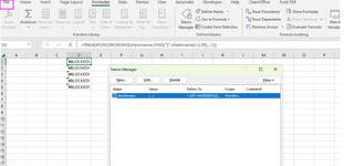
I found a related topic on #Blocked error as discussed here (I tried the function mentioned in that topic, too). The error happened maybe because my updated Office 365 has no longer supported for those functions.
 
Upvote 0

Excel Facts

Which Excel functions can ignore hidden rows?
The SUBTOTAL and AGGREGATE functions ignore hidden rows. AGGREGATE can also exclude error cells and more.
I found a related topic on #Blocked error as discussed here (I tried the function mentioned in that topic, too). The error happened maybe because my updated Office 365 has no longer supported for those functions.
We are using is not the same 365, maybe.
Click file, option, trust center, trust center setting, macro setting, Enable Excel 4.0 macros when VBA macros are enabled. Then save the book and open it. Try it.
 

Attachments

  • 1690254969422.png
    1690254969422.png
    178.8 KB · Views: 6
Upvote 0
We are using is not the same 365, maybe.
Click file, option, trust center, trust center setting, macro setting, Enable Excel 4.0 macros when VBA macros are enabled. Then save the book and open it. Try it.
Thanks to "enabling Excel 4.0 macros when VBA macros are enabled", your code worked to list all sheet names.
However, it should be pointed out that unless I have changed the last number from -1 to 1, the fomular only listed 2 first sheet names including 'Master'. Maybe because 'Master' in my case is the very first sheet.
This is it:
Book1.xlsm
ABCDE
1Master
2#REF!AhjfaweDb
3#REF!
4#REF!
5#REF!
6#REF!
7#REF!
8
Master
Cell Formulas
RangeFormula
D1:D2D1=TRANSPOSE(DROP(MID(sheetname,FIND("]",sheetname)+1,99),,-1))
B2:B7B2=SUM(REDUCE({""},D$1:D$7,LAMBDA(x,y,VSTACK(x,INDIRECT(y&"!r"&ROW()&"c1",)*INDIRECT(y&"!r"&ROW()&"c2",)))))
Dynamic array formulas.


When I change to 1, the fomular to list sheet names worked, however, the other fomular did not:
Book1.xlsm
ABCDE
1AhjfaweDb
2#REF!Dxoawe98
3#REF!
4#REF!
5#REF!
6#REF!
7#REF!
8
Master
Cell Formulas
RangeFormula
D1:D2D1=TRANSPOSE(DROP(MID(sheetname,FIND("]",sheetname)+1,99),,1))
B2:B7B2=SUM(REDUCE({""},D$1:D$7,LAMBDA(x,y,VSTACK(x,INDIRECT(y&"!r"&ROW()&"c1",)*INDIRECT(y&"!r"&ROW()&"c2",)))))
Dynamic array formulas.
 
Upvote 0
Thanks to "enabling Excel 4.0 macros when VBA macros are enabled", your code worked to list all sheet names.
However, it should be pointed out that unless I have changed the last number from -1 to 1, the fomular only listed 2 first sheet names including 'Master'. Maybe because 'Master' in my case is the very first sheet.
This is it:
Book1.xlsm
ABCDE
1Master
2#REF!AhjfaweDb
3#REF!
4#REF!
5#REF!
6#REF!
7#REF!
8
Master
Cell Formulas
RangeFormula
D1:D2D1=TRANSPOSE(DROP(MID(sheetname,FIND("]",sheetname)+1,99),,-1))
B2:B7B2=SUM(REDUCE({""},D$1:D$7,LAMBDA(x,y,VSTACK(x,INDIRECT(y&"!r"&ROW()&"c1",)*INDIRECT(y&"!r"&ROW()&"c2",)))))
Dynamic array formulas.


When I change to 1, the fomular to list sheet names worked, however, the other fomular did not:
Book1.xlsm
ABCDE
1AhjfaweDb
2#REF!Dxoawe98
3#REF!
4#REF!
5#REF!
6#REF!
7#REF!
8
Master
Cell Formulas
RangeFormula
D1:D2D1=TRANSPOSE(DROP(MID(sheetname,FIND("]",sheetname)+1,99),,1))
B2:B7B2=SUM(REDUCE({""},D$1:D$7,LAMBDA(x,y,VSTACK(x,INDIRECT(y&"!r"&ROW()&"c1",)*INDIRECT(y&"!r"&ROW()&"c2",)))))
Dynamic array formulas.
Excel Formula:
=SUM(REDUCE("",D$1#,LAMBDA(x,y,VSTACK(x,INDIRECT(y&"!r"&ROW()&"c1",)*INDIRECT(y&"!r"&ROW()&"c2",)))))
 
Upvote 0
How about
Book1 new.xlsm
ABCD
1ResultAhjfaweDb
2162.9742Dxoawe98
3164.1468
4183.3545
556.9415
667.34673
765.36402
Master
Cell Formulas
RangeFormula
D1:D2D1=TOCOL(DROP(TEXTAFTER(sheetname,"]"),,1))
A2:A7A2=SUM(REDUCE("",D$1#,LAMBDA(x,y,VSTACK(x,INDIRECT(y&"!r"&ROW()&"c1",)*INDIRECT(y&"!r"&ROW()&"c2",)))))
Dynamic array formulas.
These functions have worked flawlessly!
Thank you so much!
By the way, could you do me a favor and tell me what I should do if I want to change the columns to calculate, for example column C and E, and start calculating from C5 and E5 position instead of A2-B2?
 
Upvote 0
Excel Formula:
=SUM(REDUCE("",D$1#,LAMBDA(x,y,VSTACK(x,INDIRECT(y&"!r"&ROW()&"c1",)*INDIRECT(y&"!r"&ROW()&"c2",)))))
Yes, this also worked with similar results as the post #24.
Thank you very much for your patience and kind help!
 
Upvote 0
How about
Book1 new.xlsm
ABCD
1ResultAhjfaweDb
2162.9742Dxoawe98
3164.1468
4183.3545
556.9415
667.34673
765.36402
Master
Cell Formulas
RangeFormula
D1:D2D1=TOCOL(DROP(TEXTAFTER(sheetname,"]"),,1))
A2:A7A2=SUM(REDUCE("",D$1#,LAMBDA(x,y,VSTACK(x,INDIRECT(y&"!r"&ROW()&"c1",)*INDIRECT(y&"!r"&ROW()&"c2",)))))
Dynamic array formulas.
I think my request will make things more complicated, so I will create another thread instead, thus please ignore my post #26.
Also, I am waiting for a VBA code solution from Mr. @Snakehips.
Again, thank you very much!
 
Upvote 0
Also, I am waiting for a VBA code solution from Mr. @Snakehips.
Sorry but I thought that you were appearing to be favouring the formula solutions.
Also, coding-wise, I cannot see an issue with the code I have given.
Does the code I have given work ( with data in cols A:B), now that you have enabled Excel 4.0 macros?
 
Upvote 0
Sorry but I thought that you were appearing to be favouring the formula solutions.
Also, coding-wise, I cannot see an issue with the code I have given.
Does the code I have given work ( with data in cols A:B), now that you have enabled Excel 4.0 macros?
Actually, I prefer the code solution since I can reused it when I need to implement more complex formular by using another macro.
Unfortunately, I run both of these codes but they still not work.
The 'Master' sheet is in the very first position.

VBA Code:
Sub Code01 ()
Dim arr As Variant, res As Variant
Dim lr As Long, mlr As Long

For Each sht In ThisWorkbook.Sheets
    If Not sht.Name = "Master" Then
        If Not lr > 1 Then
            lr = sht.Cells(Rows.Count, 1).End(xlUp).Row
            ReDim arr(1 To lr - 1, 1 To 1)
            ReDim res(1 To lr - 1)
        End If
    arr = sht.Range("A2:B" & lr).Value
        For c = 1 To lr - 1
            res(c) = res(c) + (arr(c, 1) * arr(c, 2))
        Next c
    End If
Next sht
With Sheets("Master")
    mlr = .Cells(Rows.Count, 1).End(xlUp).Row
    .Range("A2:A" & mlr).ClearContents
    .Range("A2:A" & lr).Value = Application.Transpose(res)
End With
End Sub

This code resulted in error 9: Subscript out of range
At line:
VBA Code:
ReDim arr(1 To lr - 1, 1 To 1)

And this code resulted in "Check that your first data sheet has data rows in column A"
VBA Code:
Sub Code_02()
Dim arr As Variant, res As Variant
Dim lr As Long, mlr As Long, c As Long
Dim sht As Worksheet

For Each sht In ThisWorkbook.Sheets
    If Not sht.Name = "Master" Then  '<<< Edit Master if name differs
        If Not lr > 1 Then
        On Error GoTo BailOut  'controled exit sub without failing
            lr = sht.Cells(Rows.Count, 1).End(xlUp).Row      '<<< 1 = column A  Edit for another column if A not applicable
            If Not lr > 1 Then MsgBox "Check that your first data sheet has data rows in column A"   '<<<<check if lr is being set correctly??????"
            ' if no data or only header row lr <= 1 then the following will error
            ReDim arr(1 To lr - 1, 1 To 1)
            ReDim res(1 To lr - 1)
        End If
    arr = sht.Range("A2:B" & lr).Value
        For c = 1 To lr - 1
            res(c) = res(c) + (arr(c, 1) * arr(c, 2))
        Next c
    End If
Next sht
With Sheets("Master")
    mlr = .Cells(Rows.Count, 1).End(xlUp).Row
    .Range("A2:A" & mlr).ClearContents
    .Range("A2:A" & lr).Value = Application.Transpose(res)
End With
BailOut:
On Error GoTo 0  'reset default error handling
End Sub

Could you please attach the resulted file that you have run macro successfully so that I can run it again on my computer?
 
Upvote 0

Forum statistics

Threads
1,215,069
Messages
6,122,959
Members
449,096
Latest member
Anshu121

We've detected that you are using an adblocker.

We have a great community of people providing Excel help here, but the hosting costs are enormous. You can help keep this site running by allowing ads on MrExcel.com.
Allow Ads at MrExcel

Which adblocker are you using?

Disable AdBlock

Follow these easy steps to disable AdBlock

1)Click on the icon in the browser’s toolbar.
2)Click on the icon in the browser’s toolbar.
2)Click on the "Pause on this site" option.
Go back

Disable AdBlock Plus

Follow these easy steps to disable AdBlock Plus

1)Click on the icon in the browser’s toolbar.
2)Click on the toggle to disable it for "mrexcel.com".
Go back

Disable uBlock Origin

Follow these easy steps to disable uBlock Origin

1)Click on the icon in the browser’s toolbar.
2)Click on the "Power" button.
3)Click on the "Refresh" button.
Go back

Disable uBlock

Follow these easy steps to disable uBlock

1)Click on the icon in the browser’s toolbar.
2)Click on the "Power" button.
3)Click on the "Refresh" button.
Go back
Back
Top