Charts with formula linked figures

[Hrishi]

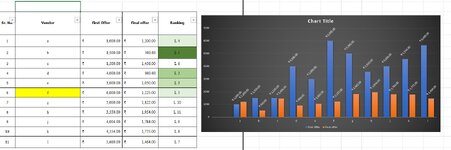
Hello, I have two queries regarding chart.
1) I have a table with figures in Rupees (INR) and i want a histograph stating figures in "LAKH" (LAkh is 1/10 million). So basically if i have value in table say 5000000.00, i want my cart to show figure 50. (50=5000000/100000)
and it should be dynamic. If i change figures in table, it should reflect in chart.

2) numbers in above table need not be sorted, but i want my histograph to be in ascending order or descending order.

pls see images attached.

 

[Hrishi]

The L 4 and L1... Is that the Lakh and is that what you want in the chart

 

[Hrishi]

The L 4 and L1... Is that the Lakh and is that what you want in the chart

Now in given example, I have generated chart in regular way. attached is the photo of it. hope its visible to you. My query is, in My chart it shows same figures what is there in table. I want chart which will show figure ( 1 / 100000) example (Final offer of vendor "a" in my table is Rupees 1200.00, so i want figure on chart (0.012). I can do this with having additional column in table. but i want to do that without any additional helper column. there should be some provision to add formula in charts, right!

secondly i don't want to sort my table in ascending order, but I want to chart in ascending order.

 

[Jimmypop]

How about...

Book1
	A	B	C	D	E	F
15	Sr. No.	Vendor	First Offer	Final offer	Lakh	Ranking
16
17	8	h	₹ 3 550.00	₹ 1 954.00	L 0.020	L 11
18	7	g	₹ 5 000.00	₹ 1 822.00	L 0.018	L 10
19	9	j	₹ 4 004.00	₹ 1 784.00	L 0.018	L 9
20	10	k	₹ 4 554.00	₹ 1 775.00	L 0.018	L 8
21	11	l	₹ 5 660.00	₹ 1 464.00	L 0.015	L 7
22	3	c	₹ 1 500.00	₹ 1 456.00	L 0.015	L 6
23	6	f	₹ 6 000.00	₹ 1 225.00	L 0.012	L 5
24	1	a	₹ 1 000.00	₹ 1 200.00	L 0.012	L 4
25	5	e	₹ 3 000.00	₹ 1 050.00	L 0.011	L 3
26	4	d	₹ 4 000.00	₹ 900.00	L 0.009	L 2
27	2	b	₹ 1 500.00	₹ 500.00	L 0.005	L 1
Approval Note

Cell Formulas
Range	Formula
E17:E27	E17	=D17/100000
F17:F27	F17	=+"L " &RANK(D17,$D$17:$D$27,1)

Named Ranges
Name	Refers To	Cells
FINALOFFER	='Approval Note'!$D$17:$D$27	F17:F27, E17

this gives chart look of



Is this correct? I do not know of another way without using helper column

 

[Hrishi]

How about...

Book1
	A	B	C	D	E	F
15	Sr. No.	Vendor	First Offer	Final offer	Lakh	Ranking
16
17	8	h	₹ 3 550.00	₹ 1 954.00	L 0.020	L 11
18	7	g	₹ 5 000.00	₹ 1 822.00	L 0.018	L 10
19	9	j	₹ 4 004.00	₹ 1 784.00	L 0.018	L 9
20	10	k	₹ 4 554.00	₹ 1 775.00	L 0.018	L 8
21	11	l	₹ 5 660.00	₹ 1 464.00	L 0.015	L 7
22	3	c	₹ 1 500.00	₹ 1 456.00	L 0.015	L 6
23	6	f	₹ 6 000.00	₹ 1 225.00	L 0.012	L 5
24	1	a	₹ 1 000.00	₹ 1 200.00	L 0.012	L 4
25	5	e	₹ 3 000.00	₹ 1 050.00	L 0.011	L 3
26	4	d	₹ 4 000.00	₹ 900.00	L 0.009	L 2
27	2	b	₹ 1 500.00	₹ 500.00	L 0.005	L 1
Approval Note

Cell Formulas
Range	Formula
E17:E27	E17	=D17/100000
F17:F27	F17	=+"L " &RANK(D17,$D$17:$D$27,1)

Named Ranges
Name	Refers To	Cells
FINALOFFER	='Approval Note'!$D$17:$D$27	F17:F27, E17

this gives chart look of

View attachment 90117

Is this correct? I do not know of another way without using helper column

out put is correct. with helper column its easy to do. it seem that you have sorted number columns in ascending order hence your are getting graph in ascending order. can we get the ascending graph without sorting column?

 

[Jimmypop]

Not sure about not using the helper column... You can always hide the column if you need ..