Checkboxes vs Drop Downs

usnapoleon

Board Regular
Joined
May 22, 2014
Messages
94
Office Version
  1. 365
Platform
  1. Windows
Hello,
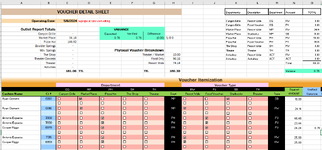
I could use an honest opinion on a project before I expend time and energy into it. I was on this forum recently getting help in making a spreadsheet where input is heavily involving checkboxes. A single tab looked like this:

1715035275554.png


There are 31 tabs total, to represent the days of the month, and 37 rows of the checkboxes per tab. One thing I noticed is that the spreadsheet was slow, and likely due to all the checkboxes.

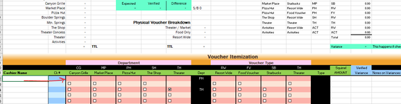
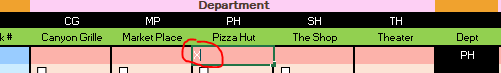
The spreadsheet works by checking 1 box on the Department area, and one box in the Voucher Type area. The black areas get populated with the checkbox-selections, and there are sumif formulas above that review the black areas and the amount $$ in the far right and bango, we have an easy-to-input spreadsheet that gives us our info. The whole intention was to make the input area easy with the use of checkboxes. It's been much easier, well received, but its nagging me that it's a slow spreadsheet, and modifying it (adding/removing checkboxes) is a pain in the butt.

What I'm envisioning is this...
1715035842853.png


We have 1 'input' area, which utilizes 2 dropdown menus you see at the top, and the amount is a simple input. you press a button, which I called above the 'post' button... and it will post the data in the area below - I color-coordinated the input sections to where they get posted, just as a visual aid. The formulas I mentioned will do sumif's based on the posted area, no biggie here. Each time you 'Post' it will apply the selected items to the next empty row. You can make edits after-the-fact, or clear data altogether if you want to redo it, etc.
  • So if you clear row 30 because of an input-accident, you can highlight the row, clear it, and the 'post' button will re-use row 30.
  • Or maybe you didnt see the input error initially, and you get to row 35 before you caught it.
    • You can delete the row entirely, which will bump up all the other rows... so 32 becomes 31, etc etc, and 35's the next blank row and your 'redo' goes there.
    • Alternatively, maybe you just cleared out row 30, so rows 29, 31-34 are populated but 30 no longer is, the Post will go there, then the next one will resume at row 35.
My questions to everyone reading...
  1. is something like this possible?
  2. will it be a faster spreadsheet?
Thank you for your time!
 

Excel Facts

Waterfall charts in Excel?
Office 365 customers have access to Waterfall charts since late 2016. They were added to Excel 2019.
Dropdowns are a personal thing. Personally I'm not a fan, but having said that I'd probably like all these checkboxes even less!

1. Yes, something like that is definitely possible
2. Hard to say if it will be faster without knowing exactly what's slowing it down currently, but most likely yes.

You would probably be able to get away without the post button if you wanted by putting some on-change event code on the amount cell that checked the other two were completed and then just posted the result before clearing the inputs again.

I've also done things before where you prompt the user for the row to put it in or by default use the next available row - that could be one way of handling your row 30 issue.
 
Upvote 0
I would never use checkboxes like this:
I would use double click sheet script.
Double click on a cell and something happens.
If this might be something you would like
Tell me what normally happens now when you click on the checkbox
 
Upvote 0
I would never use checkboxes like this:
I would use double click sheet script.
Double click on a cell and something happens.
If this might be something you would like
Tell me what normally happens now when you click on the checkbox
Hello, sorry for the delay. The Dentist held me for 5 hours today! Let me show you what happens when you click a checkbox

1715137880366.png


When you click on a box...

The department code and voucher type code from row 20 are populated in the black columns depending on what box gets selected. Row 22 above, in the black areas, has MP for the Dept and SB for the Type, and that is due to the boxes checked for each section.
  • Department black has a formula like this: =IFERROR(INDEX($C$20:$G$20,MATCH(TRUE,C22:G22,0)),"")
  • Voucher black has a formula like this: =IFERROR(INDEX($I$20:$L$20,MATCH(TRUE,I22:L22,0)),"")

The formulas in column O (top right of screenshot) sum the amounts below (less variances). They match the codes in the blank to against the codes in columns M and N.
  • The formula looks like this: =SUM(FILTER($N$21:$N$57-$O$21:$O$57,($H$21:$H$57=M4)*($M$21:$M$57=N4),0))

Thank you again for looking at this. Let me know if you have other questions!

Towards your other question, I have never heard of double click sheet script. When I googled it, it brought up Pivot tables, which didnt quite make sense. I'm all for learning something new if it's effective, easy to manage (unlike checkboxes) and able to be easily edited when rows or columns need to be added/moved/etc. In the end, I'm just trying to give my team something that makes their inputs faster. They used to do a manual input in every cell. The checkboxes allowed me to cut some of that input out, and I could do the formulas in the top right as a result. I'm always open to doing better.
 

Attachments

  • 1715137306489.png
    1715137306489.png
    72.4 KB · Views: 6
Upvote 0
If I understand correctly, instead of all these formulas I would use Vba,
This here is a Vba script that will run when you double click on a cell.
In my script the script will run when you double click on columns 3 to 7
And the results will be entered into column 8
This script runs when you double click on any cell in row greater then 21

Now if this will work for you, I can modify the script to also work on the other columns.
But let's start with this

A Vba script will only work on a workbook that is Vba enabled.

To install this script right click on the sheet Tab and choose View code and paste this code.

The script runs when you double click on any cell in columns 3 to 7 starting in row 22
VBA Code:
Private Sub Worksheet_BeforeDoubleClick(ByVal Target As Range, Cancel As Boolean)
   Application.ScreenUpdating = False
 Application.EnableEvents = False

    If Target.Row > 21 Then
    
        Select Case Target.Column
            Case 3: Target.Offset(, 5).Value = "CG": Target.Value = "X"
            Case 4: Target.Offset(, 4).Value = "MP": Target.Value = "X"
            Case 5: Target.Offset(, 3).Value = "PH": Target.Value = "X"
            Case 6: Target.Offset(, 2).Value = "SH": Target.Value = "X"
            Case 7: Target.Offset(, 1).Value = "??": Target.Value = "X"
        
        End Select
    End If

Application.ScreenUpdating = True
Application.EnableEvents = True


End Sub
 
Upvote 0
@usnapoleon
Could you please upload a sample workbook (without sensitive data) to a file-sharing site like Dropbox.com or Google Drive, and then share the link here? Also, ensure that the link is accessible to anyone.

There are 31 tabs total, to represent the days of the month, and 37 rows of the checkboxes per tab.
That's a lot.
Just an idea: How about using a Userform with checkboxes? You would only need one Userform for all sheets. Also, allowing many users to enter data directly on the sheet is more prone to causing errors which could ruin the sheet, whereas using a Userform could minimize them.
 
Upvote 0
If I understand correctly, instead of all these formulas I would use Vba,
This here is a Vba script that will run when you double click on a cell.
In my script the script will run when you double click on columns 3 to 7
And the results will be entered into column 8
This script runs when you double click on any cell in row greater then 21

Now if this will work for you, I can modify the script to also work on the other columns.
But let's start with this

A Vba script will only work on a workbook that is Vba enabled.

To install this script right click on the sheet Tab and choose View code and paste this code.

The script runs when you double click on any cell in columns 3 to 7 starting in row 22
VBA Code:
Private Sub Worksheet_BeforeDoubleClick(ByVal Target As Range, Cancel As Boolean)
   Application.ScreenUpdating = False
 Application.EnableEvents = False

    If Target.Row > 21 Then
   
        Select Case Target.Column
            Case 3: Target.Offset(, 5).Value = "CG": Target.Value = "X"
            Case 4: Target.Offset(, 4).Value = "MP": Target.Value = "X"
            Case 5: Target.Offset(, 3).Value = "PH": Target.Value = "X"
            Case 6: Target.Offset(, 2).Value = "SH": Target.Value = "X"
            Case 7: Target.Offset(, 1).Value = "??": Target.Value = "X"
       
        End Select
    End If

Application.ScreenUpdating = True
Application.EnableEvents = True


End Sub

This was very interesting. So I used an existing tab, added the VBA like you mentioned. I deleted the checkboxes in the top row so I could test. Double-clicking the box produced the desired department initials in the black column (column 8). Double clicking puts the target value of X in the cell, which resulted in column 8 showing the PH value. Weirdly, my formula in column 8 got overwritten by the PH.

1715801577279.png


It looks like... correct me if I'm wrong... if we wanted to add new columns for different departments, then it's just a revision of the code attached to the excel Tab, to add a Case 8, Case 9, etc, and inputting the specific Value in the same way you have CG, MP, etc. That seems like it would quite easily allow spreadsheet modifications in the future. Adding rows down below if we have an excessive number of vouchers would be a piece of cake, and the hassles of checkboxes (for example, the manual task of doing the 'Format Control' edit on every new checkbox) would be gone. But the most important modification would be the addition of new columns for either additional Departments or additional Voucher Types. I know next to nothing about VBA, but each 'Case' seems to correspond to a column # (is that coincidence?), so if I add an additional column for a new department (like MS for example), my guess is that this particular section of coding will look like :


VBA Code:
            Case 3: Target.Offset(, 6).Value = "CG": Target.Value = "X"
            Case 4: Target.Offset(, 5).Value = "MP": Target.Value = "X"
            Case 5: Target.Offset(, 4).Value = "PH": Target.Value = "X"
            Case 6: Target.Offset(, 3).Value = "SH": Target.Value = "X"
            Case 7: Target.Offset(, 2).Value = "MS": Target.Value = "X"
            Case 8: Target.Offset(, 1).Value = "??": Target.Value = "X"

I have some questions I hope you can help me with, and thank you in advance if you're able to:

  1. How does the VBA script direct the intended value to populate column 8?
    • I noticed that my formulas in column 8 got overwritten when I double-clicked on any of the columns 3-7, and the 'value' of the cell seems to be hard-keyed into column 8. No biggie about the formula disappearing, I just dont see anything in the VBA that stands out to explain the output value being in column 8
    • knowing this will help me understand how to do the double-click for the 2nd grouping of stuff, the 'Voucher Type' columns which currently occupy columns 9-12 with an output on the black column 13
  2. It does feel strange though to see nothing showing up in columns 3-7, and this phantom PH appear in column 8. I know there is an 'invisible' X when you double click, but is there anything more visual we can do?
    • 1715802687612.png
  3. I can see that double-clicking on a different column will change what shows up in column 8, such as clicking column 3 will change column 8 to CG. But what if I want to simply undo everything? Unchecking a checkbox would make column 8 blank again, but there doesn't seem to be a mechanism to undo a double-clicked box. I can only surmise we just highlight columns 3-8 on that row, press delete and redo?
I am liking everything I see, but I am lingering on those above questions. I almost asked how the 2nd group will look, haha. Then I re-read your email that said you'd help on it if we liked what we see. I think we're almost to that point once I get a better understanding on those questions.

You rock by the way, this is very interesting!!!
 

Attachments

  • 1715801536518.png
    1715801536518.png
    43 KB · Views: 0
  • 1715802603813.png
    1715802603813.png
    4.9 KB · Views: 0
Upvote 0
First you said:
Double clicking puts the target value of X in the cell, which resulted in column 8 showing the PH value. Weirdly, my formula in column 8 got overwritten by the PH.
Thats true entering the x will delete the formula. If this is a problem what else do you suggest?

If you try understanding the script it should help making changes.

For example, if target. Column means what column you double click on
and offset means how many columns to the right you want the result in.

So, for example if your checkbox use to be in column 20
Your script would be if target. Column = 20 then target. Offset (12).value= "MM" for example meaning column 32

Now to remove the x on all rows and columns
Do you mean all rows and all columns in the whole sheet?
Not sure I answered all your questions. If not, this may help. If not write back.

Your response was very helpful in understanding the script further!

With the formula in column 8 being overwritten, no problem there, just something I observed. Reading the rest of your response helped explain why and how this happens.

Case is defined as the Target.Column, so it's no coincidence that everything starts on column 3 and our script starts on Case 3. This confirms that adding columns will be easy!!

Now I understand better the significance of numbers like 5 here "Target.Offset(, 5)". That is how column 8 gets populated! Column 3, plus the 5, results show up in column 8... genius!

To talk about the matter of 'deleting'. I was looking at deleting input mistakes. Allow me to provide an example for clarity:
Let's say the user had 3 vouchers, so they populate rows 22, 23, and 24. But then they accidently double click on row 25.​
  • I'm sure they could click 'undo' on the spreadsheet, but what if they have progressed way beyond before they catch that error? How would they go about to get rid of their accident in row 25? There doesn't seem to be a way to reverse the input, like how unchecking a box would. My only thought is they need to highlight that cell on row 25, and the output cell in column 8 of row 25, and press the delete button (or just highlight the range of columns 3-8 of row 25 and press delete, whichever the user finds faster/easier). Is that how it should be done or is there something I'm not thinking of (other than deleting the row entirely, hahaha!)

There is one thing we didnt touch upon, the visual aspect of it. I get there is an invisible 'x' there based on the double-click. Is there anything we can do visually to show the cell selection?

By the way, I am loving this, so I say let's push forward towards addressing the 2nd group of columns (Voucher Type). Also, thank you for the helpful information in understanding the code. I don't feel lost on this at all.

I am thinking for the 2nd group of columns, we just match the case and desired target offset. Let me tackle the first one:
VBA Code:
Case 9: Target.Offset(, 4).Value = "RW": Target.Value = "X"

Aaaamazing!
 
Upvote 0
If you want to delete the X
you could use something like this:

Double click on any of these columns and the X will be removed:
In this script modify to your needs:
3, 5, 7, 8, 14, 18
The script will delete the X from and row in columns 3, 5, 7, 8, 14, 18
Your response was very helpful in understanding the script further!

With the formula in column 8 being overwritten, no problem there, just something I observed. Reading the rest of your response helped explain why and how this happens.

Case is defined as the Target.Column, so it's no coincidence that everything starts on column 3 and our script starts on Case 3. This confirms that adding columns will be easy!!

Now I understand better the significance of numbers like 5 here "Target.Offset(, 5)". That is how column 8 gets populated! Column 3, plus the 5, results show up in column 8... genius!

To talk about the matter of 'deleting'. I was looking at deleting input mistakes. Allow me to provide an example for clarity:
Let's say the user had 3 vouchers, so they populate rows 22, 23, and 24. But then they accidently double click on row 25.​
  • I'm sure they could click 'undo' on the spreadsheet, but what if they have progressed way beyond before they catch that error? How would they go about to get rid of their accident in row 25? There doesn't seem to be a way to reverse the input, like how unchecking a box would. My only thought is they need to highlight that cell on row 25, and the output cell in column 8 of row 25, and press the delete button (or just highlight the range of columns 3-8 of row 25 and press delete, whichever the user finds faster/easier). Is that how it should be done or is there something I'm not thinking of (other than deleting the row entirely, hahaha!)

There is one thing we didnt touch upon, the visual aspect of it. I get there is an invisible 'x' there based on the double-click. Is there anything we can do visually to show the cell selection?

By the way, I am loving this, so I say let's push forward towards addressing the 2nd group of columns (Voucher Type). Also, thank you for the helpful information in understanding the code. I don't feel lost on this at all.

I am thinking for the 2nd group of columns, we just match the case and desired target offset. Let me tackle the first one:
VBA Code:
Case 9: Target.Offset(, 4).Value = "RW": Target.Value = "X"

Aaaamazing!
So I'm thinking all is well now and you have this working the way you want is that correct?
I did not understand this:
You said:
There is one thing we didnt touch upon, the visual aspect of it. I get there is an invisible 'x' there based on the double-click. Is there anything we can do visually to show the cell selection?
what is an invisible X?


Now I could add to this, and the script could delete the X if you want.
It would popup an input box and would ask "Enter X or Delete X
Would you like something like that added.
 
Upvote 0

Forum statistics

Threads
1,216,102
Messages
6,128,849
Members
449,471
Latest member
lachbee

We've detected that you are using an adblocker.

We have a great community of people providing Excel help here, but the hosting costs are enormous. You can help keep this site running by allowing ads on MrExcel.com.
Allow Ads at MrExcel

Which adblocker are you using?

Disable AdBlock

Follow these easy steps to disable AdBlock

1)Click on the icon in the browser’s toolbar.
2)Click on the icon in the browser’s toolbar.
2)Click on the "Pause on this site" option.
Go back

Disable AdBlock Plus

Follow these easy steps to disable AdBlock Plus

1)Click on the icon in the browser’s toolbar.
2)Click on the toggle to disable it for "mrexcel.com".
Go back

Disable uBlock Origin

Follow these easy steps to disable uBlock Origin

1)Click on the icon in the browser’s toolbar.
2)Click on the "Power" button.
3)Click on the "Refresh" button.
Go back

Disable uBlock

Follow these easy steps to disable uBlock

1)Click on the icon in the browser’s toolbar.
2)Click on the "Power" button.
3)Click on the "Refresh" button.
Go back
Back
Top