Choose cells that come closest to adding up to a certain total

melodramatic

Board Regular
Joined
Apr 28, 2003
Messages
180
Office Version
  1. 365
Platform
  1. Windows
This is probably the strangest query I've put before you, and I think it's probably a dud. But, I'm hoping that someone can prove me wrong.

I am in charge of our daily lunch here at work, and break that lunch down on my credit card according to how many people from our two buildings (A&D) were on the lunch list. Accordingly, I charge out per the average meal cost against the number per building.

All has worked well since I took on this task a year ago. UNTIL, I.T. let some wonder-consultant change out all of our accounting software. I am no longer able to go into each charge and split it to different accounts - every single charge can go to only one charge code now. So much for splitting.

Luckily, I do my charge-outs only once a month (and that day is coming up on Wednesday, when May ends). What I'm planning on doing is taking the total of the charges for the month (using the April figures here, that was $1,425.10 for Bldg A, and $2,710.06 for Bldg D), and pulling receipts that match closest to that amount. Yes, the shortcut system that we now have in accounting takes us all 4x the amount of time to do accounting work.

Sorry, I digress in my frustration.

So, is there a way that I can tell Excel - "hey - if you look at the "A Charge" column in the table, (starting at Row 3, you're in a table), find me the receipts that will bring me the closest to $1,425.10?

Thanks in advance for looking at this!

$4,135.16$1,425.10$2,710.06
04-22AD
DateVendorType Meal# MealsA #D #ChargeA ChargeD Charge
04/04/22 (Mon)ZaxbysChicken21714$200.88
$66.96​
$133.92​
04/06/22 (Wed)Romeros Las BrazasMexican18612$275.84
$91.95​
$183.89​
04/07/22 (Thu)First Class BBQBBQ21615$255.60
$73.03​
$182.57​
04/08/22 (Fri)Every BelliesPotatoes & Burgers19712$267.11
$98.41​
$168.70​
04/11/22 (Mon)Chick-fil-AChicken Sandwiches, Wraps & Salads16511$187.06
$58.46​
$128.60​
04/12/22 (Tue)SchlotzskysSandwiches19712$250.04
$92.12​
$157.92​
04/13/22 (Wed)Joes Italian GrillItalian23914$319.09
$124.86​
$194.23​
04/14/22 (Thu)French QuarterCajun20713$325.41
$113.89​
$211.52​
04/18/22 (Mon)Backyard GrillAmerican (w/seafood)16313$224.46
$42.09​
$182.37​
04/19/22 (Tue)McAlisters DeliSandwiches19613$226.50
$71.53​
$154.97​
04/20/22 (Wed)Yangs KitchenChinese271116$281.71
$114.77​
$166.94​
04/21/22 (Thu)Classic Events CafeBurgers, etc.20614$256.29
$76.89​
$179.40​
04/22/22 (Fri)SmashburgerBurgers, etc.17611$222.94
$78.68​
$144.26​
04/25/22 (Mon)ZaxbysChicken261412$260.39
$140.21​
$120.18​
04/26/22 (Tue)Jersey MikesSandwiches21417
$0.00​
$0.00​
04/27/22 (Wed)Romeros Las BrazasMexican24816$353.41
$117.80​
$235.61​
04/28/22 (Thu)First Class BBQBBQ18513$228.43
$63.45​
$164.98​
04/29/22 (Fri)Every BelliesPotatoes & Burgers20614
$0.00​
$0.00​
 

Excel Facts

Which Excel functions can ignore hidden rows?
The SUBTOTAL and AGGREGATE functions ignore hidden rows. AGGREGATE can also exclude error cells and more.
There is a way to do this, and it's been posted here before. I believe @shg had addressed it well. It may be here...or a somewhat related post:
If I recall correctly, it involved a script that would examine all combinations of numbers provided and then determine which ones summed to a target value. These partitions were then returned by the script.

Which version of Excel are you using?...could you update your account details with that, please?
 
Upvote 0
As a follow up, what type of information is known to you then? It sounds as if you have either a pile or list of receipts. What information is conveyed by those receipts? Perhaps just Date, Vendor, and Charge? I'm assuming there is no indication whether it is an A charge or a D charge, but am not sure based on your description. I also don't know whether the receipt shows how many meals are included in the charge on that receipt. I ask because the answer to the example that you've posted for April is "all of them"...all of the A Charges are needed to sum to $1425.10, but I'm trying to understand what the initial scenario looks like that needs to be unraveled.
 
Upvote 0
KRice3, I looked at shg's posting - the problem I have with that one is that it gave a definite number to meet that sum - choose 6 numbers that add up to this. Mine has an uncertain number to be met.

As far as the information, what I get from all of my vendors is the receipt. If we look at 4/4, that receipt from Zaxbys was $200.88, for 21 people. Since 7 of those folks were Bldg. A, Bldg. A would pay 1/3 of the bill, or $66.96, leaving the balance for Bldg. D, who had 14 folks for $133.92. Each day, the receipt itself should be split between the billing codes for Bldgs. A & D, so that each building pays its share of that lunch order.

The problem we have is that our new accounting software, for the portion that I turn in, does not allow me to split receipts. Thus, what I need to do is figure out what each building should be paying for he whole month, and then find a grouping of receipts that meets up, as closely as possible, that number - charging those receipt groupings separately to each building.

For instance, on the April expenses, I went thru and hi-lited, adding and removing the total charge cells, until I got close to my amounts. How I actually charged the April is shown below. I had to charge receipts to only one building, so all yellow receipts went to D, and all pink receipts went to A, bringing the receipts to a total as close as I could to what it would have been had I been able to properly split each receipt.

But, after first hoping that whoever is in charge of our software gets around to making this change, I'm hoping there's a way I can find an easier path for getting the billing out. If not, I'll continue to pick up and drop while watching the sum in the bottom corner of my screen - but you can't blame me for hoping I can get lucky with a formula.

Thanks for taking your time on this!
 

Attachments

  • Capture.PNG
    Capture.PNG
    51.9 KB · Views: 25
Upvote 0
Interesting...and I don't need to tell you that the approach you describe makes no sense, since every meal on a vendor's receipt is not likely to be from people in only one of the buildings. Is there any possibility that your accounting software and policies would allow you to manually perform the split by reusing the same receipt twice, but designating it slightly differently? For example, on 4/4/22, instead of Zaxby's $200.88 billed against Building D, could you have a Zaxby's-A in the amount of $66.96 billed against Building A, and a Zaxby's-D in the amount of 133.92 billed against Building D? Although this breakdown isn't necessarily correct either, right? As you mentioned in your 1st post, this breakdown is based on applying an average meal cost to all customers on that day. So you know what?...the vendor, the number of customers and their corresponding building, and the total charged amount for each day?

And are you saying that there is some type of enforcement such that the accounting system will only accept a transaction in the full amount of the receipt, so the Zaxby's-A and Zaxby's-D idea cannot be made to work?

Alternatively, do the food vendors know which buildings their customers belong to? Could they possibly track it and issue two receipts every month: one for Bldg A, the other for Bldg D?

About the script, I'll post what I was thinking about. That version does not require the user to specify the number of addends, but I think it does require an exact sum...which would still be a problem in this case. Excel's Solver might be another option. Is the April example fairly typical of the scale of the problem...that is, there are about 20 work days in a month and you have only one vendor per day, so you have about 20 receipts that need to be grouped and summed to minimize the differences when compared to a weighted split of the total cost.
 
Upvote 0
Here is one approach using Excel's built-in Solver. The worksheet looks like this initially:
MrExcel_20220531_CombinationalSum_v1.xlsm
ABCDEFGHIJKL
1$4,135.16$1,425.10$2,710.061232424135.161425.102710.061920.172214.99SSD
2Apr-22AD700.134708
3DateVendorType Meal# MealsADChargeA ChargeD ChargeSelect ASelect D
404/04/22 (Mon)ZaxbysChicken21714200.8866.96133.9210
504/06/22 (Wed)Romeros Las BrazasMexican18612275.8491.95183.8901
604/07/22 (Thu)First Class BBQBBQ21615255.6073.03182.5710
704/08/22 (Fri)Every BelliesPotatoes & Burgers19712267.1198.41168.7001
804/11/22 (Mon)Chick-fil-AChicken Sandwiches, Wraps & Salads16511187.0658.46128.6010
904/12/22 (Tue)SchlotzskysSandwiches19712250.0492.12157.9201
1004/13/22 (Wed)Joes Italian GrillItalian23914319.09124.86194.2310
1104/14/22 (Thu)French QuarterCajun20713325.41113.89211.5201
1204/18/22 (Mon)Backyard GrillAmerican (w/seafood)16313224.4642.09182.3710
1304/19/22 (Tue)McAlisters DeliSandwiches19613226.5071.53154.9701
1404/20/22 (Wed)Yangs KitchenChinese271116281.71114.77166.9410
1504/21/22 (Thu)Classic Events CafeBurgers, etc.20614256.2976.89179.4001
1604/22/22 (Fri)SmashburgerBurgers, etc.17611222.9478.68144.2610
1704/25/22 (Mon)ZaxbysChicken261412260.39140.21120.1801
1804/26/22 (Tue)Jersey MikesSandwiches214170.000.000.0010
1904/27/22 (Wed)Romeros Las BrazasMexican24816353.41117.80235.6101
2004/28/22 (Thu)First Class BBQBBQ18513228.4363.45164.9810
2104/29/22 (Fri)Every BelliesPotatoes & Burgers206140.000.000.0001
Sheet1
Cell Formulas
RangeFormula
E1:I1E1=SUM(E4:E21)
J1:K1J1=SUMPRODUCT(J4:J21,$G4:$G21)
L2L2=SQRT((H1-J1)^2+(I1-K1)^2)
K4:K21K4=--NOT(J4)
Named Ranges
NameRefers ToCells
solver_adj=Sheet1!$J$4:$J$21J1, K4
solver_lhs1=Sheet1!$J$4:$J$21J1, K4

Then after running, the results were:
MrExcel_20220531_CombinationalSum_v1.xlsm
ABCDEFGHIJKL
1$4,135.16$1,425.10$2,710.061232424135.161425.102710.061425.162710.00SSD
2Apr-22AD0.08485281
3DateVendorType Meal# MealsADChargeA ChargeD ChargeSelect ASelect D
404/04/22 (Mon)ZaxbysChicken21714200.8866.96133.9201
504/06/22 (Wed)Romeros Las BrazasMexican18612275.8491.95183.8901
604/07/22 (Thu)First Class BBQBBQ21615255.6073.03182.5701
704/08/22 (Fri)Every BelliesPotatoes & Burgers19712267.1198.41168.7010
804/11/22 (Mon)Chick-fil-AChicken Sandwiches, Wraps & Salads16511187.0658.46128.6001
904/12/22 (Tue)SchlotzskysSandwiches19712250.0492.12157.9201
1004/13/22 (Wed)Joes Italian GrillItalian23914319.09124.86194.2301
1104/14/22 (Thu)French QuarterCajun20713325.41113.89211.5210
1204/18/22 (Mon)Backyard GrillAmerican (w/seafood)16313224.4642.09182.3701
1304/19/22 (Tue)McAlisters DeliSandwiches19613226.5071.53154.9701
1404/20/22 (Wed)Yangs KitchenChinese271116281.71114.77166.9401
1504/21/22 (Thu)Classic Events CafeBurgers, etc.20614256.2976.89179.4010
1604/22/22 (Fri)SmashburgerBurgers, etc.17611222.9478.68144.2610
1704/25/22 (Mon)ZaxbysChicken261412260.39140.21120.1801
1804/26/22 (Tue)Jersey MikesSandwiches214170.000.000.0001
1904/27/22 (Wed)Romeros Las BrazasMexican24816353.41117.80235.6110
2004/28/22 (Thu)First Class BBQBBQ18513228.4363.45164.9801
2104/29/22 (Fri)Every BelliesPotatoes & Burgers206140.000.000.0001
Sheet1
Cell Formulas
RangeFormula
E1:I1E1=SUM(E4:E21)
J1:K1J1=SUMPRODUCT(J4:J21,$G4:$G21)
L2L2=SQRT((H1-J1)^2+(I1-K1)^2)
K4:K21K4=--NOT(J4)
Named Ranges
NameRefers ToCells
solver_adj=Sheet1!$J$4:$J$21J1, K4
solver_lhs1=Sheet1!$J$4:$J$21J1, K4

The setup using Data > Solver looks like this:
1654012536721.png

I've set up a single cell (the Objective cell) to minimize (yellow cell at L2), which calculates the square root of the sum of squared differences between the (target A and solution A) sums and the (target D and solution D) sums. Be sure to set up the Constraints to point to the blue range (the entire range of your initial guesses. As you can see in the 1st minisheet, I simply alternate the guesses initially and then allow the optimization engine to find a solution that minimizes cell L2. I would recommend trying the Evolutionary solving method...that yielded a solution after about 43 seconds on my system. As for the other available optimization engines, I haven't set up the problem correctly for the Simplex LP option, and I didn't have any luck with the GRG Nonlinear...although I haven't investigated that yet. After processing, a popup window will ask if you'd like to keep Solver's solution, and if you accept, your initial guesses (blue cells) will be overwritten with 1's and 0's...the 1's indicating which lines are considered in creating the sum at the top of the column. You may get different solutions if the scenario is rerun, but all solutions should generate Objective cell results that are fairly small.
 

Attachments

  • 1654011636284.png
    1654011636284.png
    92.9 KB · Views: 11
Upvote 0
KRice, our new accounting system sucks. Plain and simple. What you talked about doing is what I've been doing since I took this position - splitting a single receipt into my 2 different accounts for which I work. I never had a problem on BST, where I could open up my charge, and either assign a single billing code, or split it to apply as many codes as I needed against it. At that point, I used my Columns H & I on that split bill. Thankfully, I made up this spreadsheet a long time ago, to assist me with the bill splits.

But comes D365, and the fact that you have to buy this app add-on and that app add-on, and somewhere, someone who KNOWS EVERYTHING, decided we didn't need those kind of things in our system. So those of us who do the work, not make the decisions, are scrambling like crazy trying to make our numbers come up to at least a semblance of what is real. What I'm now having to do is work it so that I can get it as close as possible. The two managers understand what's going on, so if I'm a few dollars off, that's not a problem.

And as far as getting my restaurants to split the bills - they deliver everything to the same location (Bldg D has the large lunchroom), and we're talking an average of 20ish meals - I do not want to harass managers who are already working with me by giving us great service by telling them they have to split the bill. Nope - especially since we have situations where I call them regularly an hour or so before delivery to do a last-minute add-on. Throwing on top of that which bill they're to add it to? That would make me the client that they start to grumble about.

Meanwhile, I'll try playing with your formulas tomorrow - it looks like it could be a definite way in to figuring this out. Thank you so much for looking at this for me!
 
Upvote 0
I'm not familiar with either of those applications, but based on what you've described that seems like a significant issue. The first link here, I believe, mentions the same problem, and apparently there are differences between importing a transaction and manually entering one...I don't know. The second describes some type of work-around about halfway down the page, but I have no idea whether that applies in your case:
I found another option for you to consider. In 2014, Tony Dallimore contributed several suggestions for tackling this type of problem at:
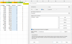
Importantly, the objective is to determine which combinations of numbers produce a sum that is either closest to a target value or within some range around a target value. The user supplies the list of starting values and the target or range. Tony describes his three offerings in terms of complexity, limitations, and general strategies for searching/solving. I am most interested in the more complex offering he describes as "Approach 3", but I have been unable to determine why it will not run for me. I also ran into difficulties with "Approach 2", although I was able to get the most basic approach working. This basic approach uses a brute-force method to determine sums of all combinations of receipts, so a major issue with it is the runtime required and whether limitations will prevent the computation of sums for tens or hundreds of millions of combinations. For that reason, if you can reduce the number of inputs, such as not using $0 receipts, that will help. In your posted example, there were 18 receipts, 2 of which were $0. I eliminated those and ran the program with 16 receipts, targeting a range of 1425.00 to 1425.20. The default setting of the program expects the initial data to be on a sheet named Source. A sheet named Results also needs to be available, as the results are written to it. I did not change the default settings, which expect the receipt data to be listed on the Source sheet in B2 and down, and in A2 and down, a unique letter code is assigned to each receipt amount. The code ran for about 2:15 (m:ss) and then returned 6 combinations satisfying the sum range condition. I then added 4 fictitious receipts (total of 20) and returned 23 minutes later to discover that it had completed, returning 22 combinations satisfying the sum range criteria. You can pick whichever combination is closest to the target. I would have guessed that reasonable estimates for runtimes would double for every receipt added: so a known 2:15 for 16 receipts...then guesses of 4:30 for 17, 9:00 for 18, 18:00 for 19, and 36:00 for 20. The fact that 20 ran in less than 23 minutes is encouraging because it may be tenable for your occasional use.

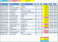
The Source sheet I used is here. Copy the block of data from your table to the white portion of the Source table, then separately copy the KeyCodes and the total Charge data into A2 and B2 (and down), respectively. Then delete any receipts/keys in the A:B columns if the value is 0...then tighten up the input data column to eliminate gaps produced by the deletions. Next, execute from the Developer menu > Macros ...the "Control" macro. You may have to add Developer to your menu bar if it is not shown. I would suggest trying this out with a very small set of receipts at first...perhaps 5 or 6, where you manually add 2 or 3 of them and establish a small range around that sum (the min and max of the range are use inputs in C3:D3). That will greatly reduce runtime and confirm that the code works on your system if it returns a combination matching your preselected receipts. I added something to the Source sheet to facilitate post-processing. After reviewing the Results sheet to identify the specific combination that you would like to use, copy the combination from the B column and paste it into G1 on the Source sheet. A formula will extract the individual letter key codes and insert 1's and 0's next to your original source data table indicating which days/vendors are part of that combination. The total shown in D13 will update based on that specific combination.
MrExcel_20220531_CombinatoricsSum.xlsm
ABCDEFGHIJKLMN
1KeyValueTarget1425.10Paste ChoiceA+D+E+G+I+J
2A200.88MinMaxA
3B275.841425.001425.20D
4C255.60E
5D267.11G
6E187.06I
7F250.04J
8G319.09
9H325.41
10I224.46
11J226.50
12K281.71Total3651232424135.161425.102710.06
13L256.291425.10UseKeyCodesDateVendor# MealsADChargeA ChargeD Charge
14M222.941A04/04/22 (Mon)Zaxbys21714200.8866.96133.92
15N260.390B04/06/22 (Wed)Romeros Las Brazas18612275.8491.95183.89
16P353.410C04/07/22 (Thu)First Class BBQ21615255.6073.03182.57
17Q228.431D04/08/22 (Fri)Every Bellies19712267.1198.41168.70
18R2251E04/11/22 (Mon)Chick-fil-A16511187.0658.46128.60
19S2000F04/12/22 (Tue)Schlotzskys19712250.0492.12157.92
20T2501G04/13/22 (Wed)Joes Italian Grill23914319.09124.86194.23
21U2750H04/14/22 (Thu)French Quarter20713325.41113.89211.52
221I04/18/22 (Mon)Backyard Grill16313224.4642.09182.37
231J04/19/22 (Tue)McAlisters Deli19613226.5071.53154.97
240K04/20/22 (Wed)Yangs Kitchen271116281.71114.77166.94
250L04/21/22 (Thu)Classic Events Cafe20614256.2976.89179.40
260M04/22/22 (Fri)Smashburger17611222.9478.68144.26
270N04/25/22 (Mon)Zaxbys261412260.39140.21120.18
280O04/26/22 (Tue)Jersey Mikes214170.000.000.00
290P04/27/22 (Wed)Romeros Las Brazas24816353.41117.80235.61
300Q04/28/22 (Thu)First Class BBQ18513228.4363.45164.98
310R04/29/22 (Fri)Every Bellies206140.000.000.00
320S  
330T  
340U  
350V  
360W  
370X  
380Y  
390Z  
Source
Cell Formulas
RangeFormula
F2:F7F2=LET(res,$G$1,str,SUBSTITUTE(res,"+",""),MID(str,ROW(INDIRECT("1:"&LEN(str))),1))
I12:N12I12=SUM(I14:I39)
D13D13=SUMPRODUCT(L14:L39,E14:E39)
M14:N39M14=IF(AND(ISNUMBER($J14:$K14)),$L14*J14/SUM($J14:$K14),"")
E14:E39E14=IF(COUNTIF($F$2#,$F14)=1,1,0)
Dynamic array formulas.

The Results sheet looks like this after running:
MrExcel_20220531_CombinatoricsSum.xlsm
AB
1TotalKey Expn
21,425.10A+D+E+G+I+J
31,425.16D+H+L+M+P
41,425.00A+C+D+F+M+Q
51,425.04C+D+I+J+M+Q
61,425.09C+D+E+J+N+Q
71,425.11A+E+H+M+N+Q
81,425.13A+C+D+F+J+R
91,425.19A+H+I+J+M+R
101,425.00D+G+N+P+R
111,425.01A+C+G+J+M+S
121,425.08A+C+J+K+N+S
131,425.17C+I+L+N+Q+S
141,425.03A+C+G+I+R+S
151,425.12A+B+D+L+R+S
161,425.19D+K+M+Q+R+S
171,425.09A+C+D+J+R+T
181,425.10E+F+K+L+S+T
191,425.14C+F+G+H+U
201,425.07B+D+H+K+U
211,425.09A+C+D+J+S+U
221,425.06E+K+L+R+S+U
231,425.10C+G+H+T+U
Result

Tony's code, modified only by changing variable types in two places based on his post advising of this correction is listed here:
VBA Code:
Option Explicit
Sub Control()

  ' Using constants instead of literals has the following effects:
  '  1) It takes longer to type the code.  For example:
  '       ValueMin = .Range(CellSrcMin).Value    takes longer to type than
  '       ValueMin = .Range("C3").Value
  '  2) The code is self-documenting.  The purpose of ".Range(CellSrcMin).Value"
  '     is a lot more obvious than the purpose of ".Range("C3").Value".  This may
  '     not matter today but, when you return to this macro in 6 months, self-
  '     documenting code is a real help.
  '  3) If a cell address, a column code or a worksheet name changes, all you
  '     have to do is change the value of the constant and the code is fixed.
  '     Scanning you code for every occurance of a literal and deciding if it
  '     one that needs to change is a nightmare.

  Const CellSrcMin As String = "C3"
  Const CellSrcMax As String = "D3"
  Const ColRsltValue As String = "A"
  Const ColRsltKeyExpn As String = "B"
  Const ColSrcKey As String = "A"
  Const ColSrcValue As String = "B"
  Const RowSrcDataFirst As Long = 2
  Const WshtNameRslt As String = "Result"
  Const WshtNameSrc As String = "Source"

  Dim InxResultCrnt As Long
  Dim InxResultPartCrnt As Long
  Dim InxSrcRowCrnt As Long
  Dim RowRsltCrnt As Long
  Dim RowSrcCrnt As Long
  Dim RowSrcDataLast As Long
  Dim SrcRows() As String
  Dim Result() As String
  Dim ResultPart() As String
  Dim ValueCrnt As Double
  Dim ValueKey As String
  Dim ValueMin As Double
  Dim ValueMax As Double

  ' Find last row containing data
  With Worksheets(WshtNameSrc)
    RowSrcDataLast = .Cells(Rows.Count, ColSrcKey).End(xlUp).Row
  End With

  ' Rows RowSrcDataFirst to RowSrcDataLast contain data.
  ' Size SrcRows so it can hold each value in this range
  ReDim SrcRows(1 To RowSrcDataLast - RowSrcDataFirst + 1)

  ' Fill SrcRows with every row that contains data
  RowSrcCrnt = RowSrcDataFirst
  For InxSrcRowCrnt = 1 To UBound(SrcRows)
    SrcRows(InxSrcRowCrnt) = RowSrcCrnt
    RowSrcCrnt = RowSrcCrnt + 1
  Next

  ' Generate every possible combination
  Call GenerateCombinations(SrcRows, Result, "|")

  ' Output contents of Result to Immediate Window.
  ' Delete or comment out once you fully understand what
  ' GenerateCombinations is doing.
  Debug.Print "Inx Combination"
  For InxResultCrnt = 0 To UBound(Result)
    Debug.Print Right("  " & InxResultCrnt, 3) & "  " & Result(InxResultCrnt)
  Next

  ' Get the minimum and maximum values
  With Worksheets(WshtNameSrc)
    ValueMin = .Range(CellSrcMin).Value
    ValueMax = .Range(CellSrcMax).Value
  End With

  ' Initialise result worksheet
  With Worksheets(WshtNameRslt)
    .Cells.EntireRow.Delete
    With .Range("A1")
      .Value = "Total"
      .HorizontalAlignment = xlRight
    End With
    .Range("B1").Value = "Key Expn"
    .Range("A1:B1").Font.Bold = True
    ' This value will be overwritten if any combination gives an acceptable value
    .Range("A2").Value = "No combination gives a value in the range " & _
                         ValueMin & " to " & ValueMax
  End With
  RowRsltCrnt = 2

  With Worksheets(WshtNameSrc)

    ' Get the minimum and maximum values
    ValueMin = .Range(CellSrcMin).Value
    ValueMax = .Range(CellSrcMax).Value

    ' For each result except first which is no row selected
    For InxResultCrnt = 1 To UBound(Result)
      ResultPart = Split(Result(InxResultCrnt), "|")
      ValueCrnt = 0#
      For InxResultPartCrnt = 0 To UBound(ResultPart)
        ValueCrnt = ValueCrnt + .Cells(ResultPart(InxResultPartCrnt), ColSrcValue).Value
      Next
      If ValueMin <= ValueCrnt And ValueMax >= ValueCrnt Then
        ' This value within acceptable range
        Worksheets(WshtNameRslt).Cells(RowRsltCrnt, ColRsltValue) = ValueCrnt
        ' Create key string
        ValueKey = .Cells(ResultPart(0), ColSrcKey).Value
        For InxResultPartCrnt = 1 To UBound(ResultPart)
          ValueKey = ValueKey & "+" & .Cells(ResultPart(InxResultPartCrnt), ColSrcKey).Value
        Next
        Worksheets(WshtNameRslt).Cells(RowRsltCrnt, ColRsltKeyExpn) = ValueKey
        RowRsltCrnt = RowRsltCrnt + 1
      End If
    Next

  End With

End Sub
Sub GenerateCombinations(ByRef Value() As String, ByRef Result() As String, _
                         ByVal Sep As String)

  ' * On entry, array Value contains values.  For example: A, B, C.
  ' * On exit, array Result contains one entry for every possible combination
  '   of values from Value.  For example, if Sep = "|":
  '     0)             ' None of the values is an allowable combination
  '     1)  A
  '     2)  B
  '     3)  A|B
  '     4)  C
  '     5)  A|C
  '     6)  B|C
  '     7)  A|B|C
  ' * The bounds of Value can be any valid range,
  ' * The lower bound of Result will be zero.  The upper bound of Result
  '   will be as required to hold all combinations.

  Dim InxRMax As Long           ' Maximum used entry in array Result
  Dim InxVRCrnt As Long         ' Working index into arrays Value and InxResultCrnt
  Dim NumValues As Long         ' Number of values
  Dim InxResultCrnt() As Long   ' Entry = 1 if corresponding value
                                ' selected for this combination

  NumValues = UBound(Value) - LBound(Value) + 1

  ReDim Result(0 To 2 ^ NumValues - 1)                 ' One entry per combination
  ReDim InxResultCrnt(LBound(Value) To UBound(Value))  ' One entry per value

  ' Initialise InxResultCrnt for no values selected
  For InxVRCrnt = LBound(Value) To UBound(Value)
    InxResultCrnt(InxVRCrnt) = 0
  Next

  InxRMax = -1
  Do While True
    ' Output current result
    InxRMax = InxRMax + 1
    If InxRMax > UBound(Result) Then
      ' There are no more combinations to output
      Exit Sub
    End If
    Result(InxRMax) = ""
    For InxVRCrnt = LBound(Value) To UBound(Value)
      If InxResultCrnt(InxVRCrnt) = 1 Then
        ' This value selected
        If Result(InxRMax) <> "" Then
          Result(InxRMax) = Result(InxRMax) & Sep
        End If
        Result(InxRMax) = Result(InxRMax) & Value(InxVRCrnt)
      End If
    Next
    ' Treat InxResultCrnt as a little endian binary number
    ' and step its value by 1.  Ignore overflow.
    ' Values will be:
    '   000000000
    '   100000000
    '   010000000
    '   110000000
    '   001000000
    '   etc
    For InxVRCrnt = LBound(Value) To UBound(Value)
      If InxResultCrnt(InxVRCrnt) = 0 Then
        InxResultCrnt(InxVRCrnt) = 1
        Exit For
      Else
        InxResultCrnt(InxVRCrnt) = 0
      End If
    Next
  Loop

End Sub
Finally, a link to the version of the file I used is here if you want to start with it:
 
Upvote 0
I figured out what I had done wrong in my earlier attempts to make Tony Dallimore's "Approach 3" work...the more complex approach I mentioned in post #8 and described in the link in that post. Tony had split the VBA listing into parts (due to posting size limitations), but those parts need to be consolidated into a single module in the VBA editor. The Source sheet setup is similar, except this approach finds solutions near a single target (a range is not specified). Your set of 16 receipts ran in less than 6 seconds. The Results sheet shows 40 combinations that are within a couple of dollars of the target. An autofilter can be quickly added to the results headings, which are then sorted by Total sum so that you can look down to find anything at or near the target (in this case 1425.00). There was one combination that produced the target sum exactly:
MrExcel_20220531_CombinatoricsSum_Approach3.xlsm
ABCD
181,425.100AE+AA+AI+AJ+AD+AG+187.06+200.88+224.46+226.5+267.11+319.09
Result

This VBA code handles Key Codes (the letter coding for each input number) up to 3-letters long. I used 2-letter key codes, and would recommend that in case you have more than 26 receipts. Be aware that the code overwrites the Results sheet, and when it does, the Total sums reported are shown rounded to the nearest integer. That column needs to be number formatted to 2 decimal places after each run. After finding the best combination, copy the Key Expn cell and paste it into Source!F1 where it will be split using one of the ATEXTSPLIT LAMBDA's posted by @Xlambda here:
This results in a nice spilling array used to populate the column to the left of the original source data so that you can easily find which rows should be included for accounting purposes. The VBA code is unchanged from what is available at the link in Post #8.
MrExcel_20220531_CombinatoricsSum_Approach3.xlsm
ABCDEFGHIJKLMNOPQ
1KeyValueTargetResults TotalPaste Choice->AE+AA+AI+AJ+AD+AG
2AE187.061425.101425.10AE3651232424135.161425.102710.06
3AA200.88AAUseKeyCodesDateVendor# MealsADChargeA ChargeD Charge
4AM222.94AI1AA04/04/22 (Mon)Zaxbys21714200.8866.96133.92
5AI224.46AJ0AB04/06/22 (Wed)Romeros Las Brazas18612275.8491.95183.89
6AJ226.50AD0AC04/07/22 (Thu)First Class BBQ21615255.6073.03182.57
7AQ228.43AG1AD04/08/22 (Fri)Every Bellies19712267.1198.41168.70
8AF250.041AE04/11/22 (Mon)Chick-fil-A16511187.0658.46128.60
9AC255.600AF04/12/22 (Tue)Schlotzskys19712250.0492.12157.92
10AL256.291AG04/13/22 (Wed)Joes Italian Grill23914319.09124.86194.23
11AN260.390AH04/14/22 (Thu)French Quarter20713325.41113.89211.52
12AD267.111AI04/18/22 (Mon)Backyard Grill16313224.4642.09182.37
13AB275.841AJ04/19/22 (Tue)McAlisters Deli19613226.5071.53154.97
14AK281.710AK04/20/22 (Wed)Yangs Kitchen271116281.71114.77166.94
15AG319.090AL04/21/22 (Thu)Classic Events Cafe20614256.2976.89179.40
16AH325.410AM04/22/22 (Fri)Smashburger17611222.9478.68144.26
17AP353.410AN04/25/22 (Mon)Zaxbys261412260.39140.21120.18
180AO04/26/22 (Tue)Jersey Mikes214170.000.000.00
190AP04/27/22 (Wed)Romeros Las Brazas24816353.41117.80235.61
200AQ04/28/22 (Thu)First Class BBQ18513228.4363.45164.98
210AR04/29/22 (Fri)Every Bellies206140.000.000.00
220AS  
230AT  
240AU  
250AV  
260AW  
270AX  
280AY  
290AZ  
Source
Cell Formulas
RangeFormula
D2D2=SUMPRODUCT(O4:O29,H4:H29)
E2:E7E2=TRANSPOSE(LAMBDA(ar,[dl],[ea], LET(d, CHAR(1),s, CHAR(2),f, CLEAN(ar),t, dl, a, SUBSTITUTE(f, t, d), b, IF(ea,a,SUBSTITUTE(SUBSTITUTE(TRIM(SUBSTITUTE(SUBSTITUTE(a, " ", s), d, " ")), " ", d),s," ")), n, LEN(b) - LEN(SUBSTITUTE(b, d, "")) + 1, m, MAX(n), c, SEQUENCE(, m), x, SEARCH(s, SUBSTITUTE(d & b, d, s, c)), y, SEARCH(s, SUBSTITUTE(b & d, d, s, c)), z, IFERROR(MID(b, x, y - x), ""), IFERROR(--z, z) ) )(F1,"+"))
L2:Q2L2=SUM(L4:L29)
P4:Q29P4=IF(AND(ISNUMBER($M4:$N4)),$O4*M4/SUM($M4:$N4),"")
H4:H29H4=IF(COUNTIF($E$2#,$I4)=1,1,0)
Dynamic array formulas.

Here is a link to my workbook if you want to avoid any setup issues. You should be able to paste any new data into the white portion of the Source sheet table, enter the Target value in C2 and then run the Macro called Control3.
 
Upvote 0
KRice3, I looked at shg's posting - the problem I have with that one is that it gave a definite number to meet that sum - choose 6 numbers that add up to this. Mine has an uncertain number to be met.

As far as the information, what I get from all of my vendors is the receipt. If we look at 4/4, that receipt from Zaxbys was $200.88, for 21 people. Since 7 of those folks were Bldg. A, Bldg. A would pay 1/3 of the bill, or $66.96, leaving the balance for Bldg. D, who had 14 folks for $133.92. Each day, the receipt itself should be split between the billing codes for Bldgs. A & D, so that each building pays its share of that lunch order.

The problem we have is that our new accounting software, for the portion that I turn in, does not allow me to split receipts. Thus, what I need to do is figure out what each building should be paying for he whole month, and then find a grouping of receipts that meets up, as closely as possible, that number - charging those receipt groupings separately to each building.

For instance, on the April expenses, I went thru and hi-lited, adding and removing the total charge cells, until I got close to my amounts. How I actually charged the April is shown below. I had to charge receipts to only one building, so all yellow receipts went to D, and all pink receipts went to A, bringing the receipts to a total as close as I could to what it would have been had I been able to properly split each receipt.

But, after first hoping that whoever is in charge of our software gets around to making this change, I'm hoping there's a way I can find an easier path for getting the billing out. If not, I'll continue to pick up and drop while watching the sum in the bottom corner of my screen - but you can't blame me for hoping I can get lucky with a formula.

Thanks for taking your time on this!
using one of the ATEXTSPLIT LAMBDA's posted by @Xlambda
Hello, melodramatic, KRice
I am here because I have received a notification that KRice mentioned one of my functions. Thank you KRice for that. Highly appreciated!!!
I also looked at the problem and I think I can solve it with a function that I have, that deals with combinatorics.
The question is, is ok with you guys if I post the solution under my thread, ARRANGEMENTS where all the study and formulas are?
Looking forward to your answer!
 
Upvote 0

Forum statistics

Threads
1,216,085
Messages
6,128,733
Members
449,465
Latest member
TAKLAM

We've detected that you are using an adblocker.

We have a great community of people providing Excel help here, but the hosting costs are enormous. You can help keep this site running by allowing ads on MrExcel.com.
Allow Ads at MrExcel

Which adblocker are you using?

Disable AdBlock

Follow these easy steps to disable AdBlock

1)Click on the icon in the browser’s toolbar.
2)Click on the icon in the browser’s toolbar.
2)Click on the "Pause on this site" option.
Go back

Disable AdBlock Plus

Follow these easy steps to disable AdBlock Plus

1)Click on the icon in the browser’s toolbar.
2)Click on the toggle to disable it for "mrexcel.com".
Go back

Disable uBlock Origin

Follow these easy steps to disable uBlock Origin

1)Click on the icon in the browser’s toolbar.
2)Click on the "Power" button.
3)Click on the "Refresh" button.
Go back

Disable uBlock

Follow these easy steps to disable uBlock

1)Click on the icon in the browser’s toolbar.
2)Click on the "Power" button.
3)Click on the "Refresh" button.
Go back
Back
Top