Compare 2 sets of data in EXCEL and return what it should be

[jezvanderbrown]

Hi everyone


I need some help with comparing 2 sets of data in Excel (see screenshot below).

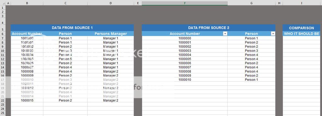
As you can see i have data from 2 sources. Source 1 is the correct data. Source 2 may have been correct at some point but its not up-to-date. I want to be able to look at the Account number and Person in Data Source 2 to see if it matches the Account Number and Person in Data Source 1.

• If it matches then i would like the cell adjacent in column I to remain blank.
• If it DOES NOT match then i would like to bring the person from Data Source 1 into the cell adjacent in column I

FYI

• The data starts from row 7 and there could be as many as 5000 Account Numbers
• If the Account Number in source 2 is not in the list of account numbers in Source 1, then i would like the word CHECK to be inserted into the cell adjacent in column I.
• I use Excel 2013

Please find a link to a copy of the spreadsheet below (hosted on Google Drive):
https://drive.google.com/file/d/0B0FUMX_fxi4GelBxS0cxTE00eHM/view?usp=sharing

I tried using 'COUNTIFS' which works to a certain extent; it compares whether they match or not but i cant figure out how to do all of the above that i need. I presume a Macro is needed but i have no clue where to start with creating a Macro to do the above.

If someone could help i'd greatly appreciate it!

Thanks in advance
Jeremy

 

[etaf]

try using
=IFERROR(IF(INDEX($C$7:$C$1000,MATCH(F7,$B$7:$B$1000,0))=G7,"",INDEX($C$7:$C$1000,MATCH(F7,$B$7:$B$1000,0))),"check")

if data 2 is blank for account ID
use

=IF(F7="","",IFERROR(IF(INDEX($C$7:$C$1000,MATCH(F7,$B$7:$B$1000,0))=G7,"",INDEX($C$7:$C$1000,MATCH(F7,$B$7:$B$1000,0))),"check"))

 

[AliGW]

In I7, copied down:

=IFNA(IF(VLOOKUP(F7,$B$7:$C$22,2)=G7,"",VLOOKUP(F7,$B$7:$C$22,2)),"check")

Extend the array to suit.

 

[wesborland1234]

I don't think you need a macro.

What you need is the MATCH function. It searches a range for a value, and returns the location relative to that range.

This should work, if your sheet is formatted just like the picture:

=IF(ISERROR(MATCH(F7,$B$7:$B$22,0)),"CHECK",OFFSET($B$7,MATCH(F7,$B$7:$B$22,0)-1,2))

Put that in I7, replace both B22's with however many rows you have. And then copy all the way down.

The IF ISERROR part, finds when an account number is not found to put "CHECK".

 

[nardagus]

Hello,

You don't need macro for this. Try this formula:

Excel 2007

Worksheet Formulas Cell Formula I7 =IF(ISERROR(MATCH($A7,$D:$D,0)),"Check",IF($B7=INDEX($E:$E,MATCH($A7,$D:$D,0)),"",IF($B7<>INDEX($E:$E,MATCH($A7,$D:$D,0)),$B7))) <tbody> </tbody>

<tbody>
</tbody>

- column A contains SRC1 account no.
- column B contains SRC1 persons
- column D contains SRC2 account no.
- column E contains SRC2 persons

What this formula does is:
1) using MATCH function checks if account no. from SRC1 exists in SRC2. If not MATCH will return an error which is TRUE for ISERROR function. Therefore first IF will return CHECK
2) Second IF will take account no. from current row in SRC1, check for its position in SRC2 with MATCH and using INDEX will return PERSON. Then it will compare PERSON from current row with PERSON returned by INDEX. If they are equal it will leave cell empty in column I
3) Third IF will do almost the same as second IF but it will check if returned PERSONS are different. If yes it will return PERSON from SRC1 (column B)

 

[jezvanderbrown]

Thanks everyone for your replies, they all pretty much do what i need so thank you very much for your help! really appreciate it!!

Jeremy

 

[AliGW]

You're welcome!