Comparing two rows in Excel for a particular word and returning the content found in that cell where the word is in a new row

[Sailadarohit]

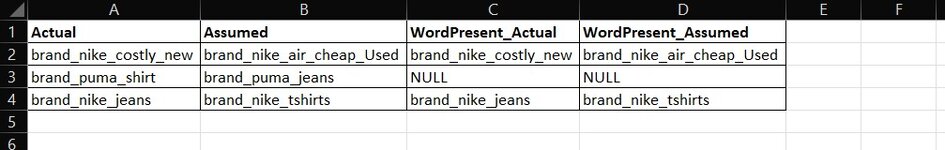
I want to compare two rows in Excel for a particular word and return the entire content found in that cell where the word is present in the new rows.
So i am searching with the word nike in the two rows, the formula should search both the rows for the word nike and if found return the entire content found along with the word nike in the new rows else return NULL.
Row A and B are my inputs, output should look like row C and D
Please refer the attachment for more information.

 

[Sailadarohit]

Unfortunately for office work i have to use 2016

What is the answer to my first question in post 28?

2016 version peter

 

[Peter_SSs]

Sailadarohit_1.xlsm
	A	B	C	D
1	Actual	Assumed	WordPresent Actual	WordPresent Assumed
2	Dress, brand_nike_costly_new, Store	Jeans, brand_nike_air_cheap_Used, Online	brand_nike_costly_new	brand_nike_air_cheap_Used
3	Online, brand_puma_shirt, Paid	Store, brand_puma_jeans, Return	NULL	NULL
4	Offline, brand_nike_jeans, Card	Shirt, brand_nike_tshirts	brand_nike_jeans	brand_nike_tshirts
5	Dress, brand_moniker_costly_new, Store	Jeans, brand_moniker_costly_new	NULL	NULL
6	black_nike_pro	black_nike_beta	black_nike_pro	black_nike_beta
7	online,black_nike_pro	black_nike_air	black_nike_pro	black_nike_air
8	offline,red_nike,pants	shop,red_nike_air,shirts	red_nike	red_nike_air
9	Dress, Hyderabad,brand_nike_costly_new, Store	Jeans, Hyd, brand_nike_air_cheap_Used, Online	brand_nike_costly_new	brand_nike_air_cheap_Used
10	Online, Banglore, Return, brand_nike_shirt, Paid	Store, Chennai, brand_nike_jeans, Return	brand_nike_shirt	brand_nike_jeans
11	online,Jeans, Hyderabad,black_nike_pro	online,Hyderabad,black_nike,shirt	black_nike_pro	black_nike
Sheet2

Cell Formulas
Range	Formula
C2:D11	C2	=IFERROR(TRIM(RIGHT(SUBSTITUTE(LEFT(A2,FIND(",",A2&",",SEARCH("_nike",A2))-1),",",REPT(" ",100)),100)),"NULL")

 

[Sailadarohit]

Thank You Peter
all the cases are addressed now

 

[Peter_SSs]

Cheers. Thanks for the confirmation.