Conditional Format Occurrences of Values In a Table

BWMagee

Board Regular
Joined
Feb 18, 2014
Messages
112
Hi,

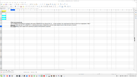
In Sheet1, A1, I enter a value. Eg. 3. This corresponds to a value in "Person ID"
In Sheet1, A3:10, I have numeric values 1, 2, 3, etc… This is “Group ID”

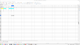
In Sheet2, A3:10, I have numeric values 1, 2, 3, etc… This is “Person ID”
In Sheet2, B3:F10, I have various numeric values. These correspond to “Group ID”

What I would like to do, using a formula in conditional formatting, is colour the values in Sheet1, A3:10, that are found in one row of the B3:F10 table. The row in which we look is determined by the value placed in Sheet1, A1.

Eg. If we enter "3" in Sheet1, A1, this means we look in row B3:F3. If the values 4, 6 and 8 are found in that row, and they are also found in Sheet1, A3:10, then we colour them using conditional formatting in Sheet1, A3:10. If Sheet1, A3:10 also contains other values that are not found in B3:F3 (eg, 5, 7 and 9), then these are not coloured.

I know how to do this when looking in a single row, but not within a table. For a single row, the formula applied to Sheet1, A3:10 in conditional formatting, would be:

=IF(COUNTIF('Sheet2'$B$3:$F$3,'Sheet1'A3),1,0)

The problem is, I will not always be looking in B3:F3, sometimes I will look in B4:F4, or B5:F5, etc… depending which value I enter into Sheet1, A1. How can I write a formula that does that?
Many thanks!
 

Excel Facts

What is the last column in Excel?
Excel columns run from A to Z, AA to AZ, AAA to XFD. The last column is XFD.
ok,
putting together a sample sheet to see if i can work out what you need

Sheet1!A1 has a number that defines the ROW number to look in , as you said
If we enter "3" in Sheet1, A1, this means we look in row B3:F3.

why 4,6,8
If we enter "3" in Sheet1, A1, this means we look in row B3:F3. If the values 4, 6 and 8 are found in that row,
I thought any number that appears in B3 to F3 , and also appears in sheet1 A3 to A10 - would highlight

FYI
in conditional formatting , you only need a TRUE FALSE - so
COUNTIF('Sheet2'$B$3:$F$3,'Sheet1'A3)
would do
I usually add the >0
COUNTIF('Sheet2'$B$3:$F$3,'Sheet1'A3)>0
to be clear
 
Upvote 0
@etaf
Thanks for your reply, but all I see is that you copied the formula I already provided, then didn't read the very next line underneath...
 
Upvote 0
that was simply to show how I use the formula you provided in a conditional formatting formula - you dont need the IF()
I also added before the formula FYI - For Your Information
So that part was information only

Maybe it would be useful if you added a sample sheets using XL2BB - so we can see what you have and also include the expected results, see my signature or on the MENU XL2BB on each reply formatting the post

the first section is where I asked some questions, as i did not understand exactly what you are doing

Here Again
1) Does the Number in A1 - Define the Row number, if so then ROW() maybe possible to use
Sheet1!A1 has a number that defines the ROW number to look in , as you said
If we enter "3" in Sheet1, A1, this means we look in row B3:F3.

2) Why are values 4,6,8 found and not just any number that happens to be in the row

why 4,6,8
If we enter "3" in Sheet1, A1, this means we look in row B3:F3. If the values 4, 6 and 8 are found in that row,
I thought any number that appears in B3 to F3 , and also appears in sheet1 A3 to A10 - would highlight
 
Upvote 0
I have attached a couple of images. Hopefully it makes it easier to understand.
 

Attachments

  • Excel Sheet1.png
    Excel Sheet1.png
    162.4 KB · Views: 21
  • Excel sheet2.png
    Excel sheet2.png
    128.8 KB · Views: 19
Upvote 0
sorry, i can not see the images easily when opening - can you use xl2bb
or put on a share ?
 
Upvote 0
ok, i'll have to have a look and see if i can recreate the spreadsheet , and offer a solution, but I have limited time on the forums for the next few days.
I can see from your example that the contents of cell A1 , does NOT match the Row
as you have row 5 highlighted because it has a 3 in the ID range
so we need to look at the number in A1 and then on sheet 2 it NOT the row 3 - we are looking up that ID number on sheet2 and using that row to compare , so a little more complicated that just using the address and row(A1)
 
Upvote 0
The images have 2560 width resolution. Should be no trouble seeing them properly.
However, you are then expecting helpers to manually type out that sample data to test with. ;)
You will generally get many more potential helpers and faster replies if you make it easier for helpers by providing sample data in a format that can quickly copy from the forum into their own test file. That is, XL2BB

This would also help:
I suggest that you update your Account details (click your user name at the top right of the forum) so helpers always know what Excel version(s) & platform(s) you are using as the best solution often varies by version. (Don’t forget to scroll down & ‘Save’)

See if this is what you want.

BWMagee.xlsm
A
13
2
31
42
53
64
75
86
97
108
Sheet1
Cells with Conditional Formatting
CellConditionCell FormatStop If True
A3:A10Expression=COUNTIF(INDEX(Sheet2!B$3:F$10,MATCH(A$1,Sheet2!A$3:A$10,0),0),A3)textNO
 
Upvote 0
Solution
if i understand correctly , it was the ROW() that the number appeared

SO I have used a complicated formula specifically setup for that example
and may not be what you want - if Peter_SSs works - then ignore mine

My logic - is to lookup which row , the number in sheet1 matches the number in $A$1 on sheet1
So if that number 3 in A1
is on row() 8 on sheet1 - A3:A50
then its matching the numbers on sheet2 that are in row 8

maybe over complicated , but as i have spent the time now looking into the issue , i thought i would post anyway - BUT as i say Peter_SSs may hav solved matching the ID on both sheets

in conditional formatting, I have selected sheet1 A3 to A10
then used
=COUNTIF(INDIRECT(ADDRESS(SUMPRODUCT(($A$3:$A$50=$A$1)*ROW($A$3:$A$50)),2,,,"sheet2")&":"&ADDRESS(SUMPRODUCT(($A$3:$A$50=$A$1)*ROW($A$3:$A$50)),6)),A3)
as a conditional formatting

Explanation
We use
SUMPRODUCT(($A$3:$A$50=$A$1)*ROW($A$3:$A$50) to find what row number in sheet1 A3 to A10 has the value matching a1
now we have the ROW() in my case 3 in A1 , matches the 3 in A3:A10 on sheet1 and is in row8
so then I add that as an address
ADDRESS(SUMPRODUCT(($A$3:$A$50=$A$1)*ROW($A$3:$A$50)),2,,,"sheet2")
this will return Sheet2!$B$8
ADDRESS(SUMPRODUCT(($A$3:$A$50=$A$1)*ROW($A$3:$A$50)),6))
Will return $F$8
and joining together with concatenate &
Sheet2!$B$8:$F$8

to use that in a formula we have to use indirect()
(INDIRECT(ADDRESS(SUMPRODUCT(($A$3:$A$50=$A$1)*ROW($A$3:$A$50)),2,,,"sheet2")&":"&ADDRESS(SUMPRODUCT(($A$3:$A$50=$A$1)*ROW($A$3:$A$50)),6))
and then I use a countif() to see if the numbers on sheet2 row 8 - column B to F
match any of the numbers in sheet1 column a3:A10

BUT IGNORE if this in not what you wanted , and simply matching the ID on both sheets, then much simplier


Sheet1
Book1
ABCDEFGHIJKLMN
13
2In Sheet1, A1, I enter a value. Eg. 3. This corresponds to a value in "Person ID" In Sheet1, A3:10, I have numeric values 1, 2, 3, etc… This is “Group ID” In Sheet2, A3:10, I have numeric values 1, 2, 3, etc… This is “Person ID” In Sheet2, B3:F10, I have various numeric values. These correspond to “Group ID”
31124
49
5143638
6103
753
837910
97
108
11
12AddressFull Equation
13Sheet2!$F$80
141
150Eg. If we enter "3" in Sheet1, A1, this means we look in row B3:F3. If the values 4, 6 and 8 are found in that row, and they are also found in Sheet1, A3:10, then we colour them using conditional formatting in Sheet1, A3:10. If Sheet1, A3:10 also contains other values that are not found in B3:F3 (eg, 5, 7 and 9), then these are not coloured.
161
170
181
191
200
210
220
230
240
250
260
Sheet1
Cell Formulas
RangeFormula
C13C13=ADDRESS(SUMPRODUCT((A3:A50=A1)*ROW(A3:A50)),6,,,"Sheet2")
D13:D26D13=COUNTIF(INDIRECT(ADDRESS(SUMPRODUCT(($A$3:$A$50=$A$1)*ROW($A$3:$A$50)),2,,,"sheet2")&":"&ADDRESS(SUMPRODUCT(($A$3:$A$50=$A$1)*ROW($A$3:$A$50)),6)),A3)
Cells with Conditional Formatting
CellConditionCell FormatStop If True
A3:A10Expression=COUNTIF(INDIRECT(ADDRESS(SUMPRODUCT(($A$3:$A$50=$A$1)*ROW($A$3:$A$50)),2,,,"sheet2")&":"&ADDRESS(SUMPRODUCT(($A$3:$A$50=$A$1)*ROW($A$3:$A$50)),6)),A3)textNO


Sheet2
Book1
ABCDEFG
1
2
31124
42
5133333
64
75
8373910
9533
108
11
Sheet2
 
Upvote 0

Forum statistics

Threads
1,215,583
Messages
6,125,661
Members
449,247
Latest member
wingedshoes

We've detected that you are using an adblocker.

We have a great community of people providing Excel help here, but the hosting costs are enormous. You can help keep this site running by allowing ads on MrExcel.com.
Allow Ads at MrExcel

Which adblocker are you using?

Disable AdBlock

Follow these easy steps to disable AdBlock

1)Click on the icon in the browser’s toolbar.
2)Click on the icon in the browser’s toolbar.
2)Click on the "Pause on this site" option.
Go back

Disable AdBlock Plus

Follow these easy steps to disable AdBlock Plus

1)Click on the icon in the browser’s toolbar.
2)Click on the toggle to disable it for "mrexcel.com".
Go back

Disable uBlock Origin

Follow these easy steps to disable uBlock Origin

1)Click on the icon in the browser’s toolbar.
2)Click on the "Power" button.
3)Click on the "Refresh" button.
Go back

Disable uBlock

Follow these easy steps to disable uBlock

1)Click on the icon in the browser’s toolbar.
2)Click on the "Power" button.
3)Click on the "Refresh" button.
Go back
Back
Top