Conditional format

[Livin404]

Good afternoon I need a little help with conditional formatting. I’m using it to identify errors before its uploaded into a large database (not Excel) I have a column where last name, first name, middle name and suffix will need to be entered. I already have it highlight punctuation marks, numbers, and spaces before or after the last name, first etc. ( none of those can be used). I used =LEN($A2)>LEN(TRIM($A2)). To flag spaces. In short. with the cell there are four blocks of information in one cell, last name, first name, and middle initial and suffix. I need the cell to highlight if there is no information after the first name.
For example my full name is:
Whiteside Sheridan Ulysses III.
In the cell I need to highlight if I only enter Whiteside Sheridan.

Thank you,

 

[sparky2205]

This will work under the strict condition that there is NO information after the first name, which is what you requested:
=ISERROR(FIND(" ",A2,FIND(" ",A2)+1))

 

[Livin404]

This will work under the strict condition that there is NO information after the first name, which is what you requested:
=ISERROR(FIND(" ",A2,FIND(" ",A2)+1))

That worked brilliantly thank you so much. Since I’m here I was wondering in one column I have a single letter to discribe the department Column F, then in another Column J I have positions that are unique to those departments. I want to pull from a list of positions. It would error out if the wrong position was typed in. If I have 5 different positions, would I create 5 name ranges. These departments have about 12 different positions?

 

[sparky2205]

Could you give me a visual representation of what you are looking for?
Would your list look like:

or maybe:

Where would you be typing in the position which would have to catch the error?

 

[Livin404]

Could you give me a visual representation of what you are looking for?
Would your list look like:
View attachment 23286
or maybe:
View attachment 23287
Where would you be typing in the position which would have to catch the error?

Like the first image. The dept will be filled then the user would type in the position. Position has to be typed there cannot be data validation dropdown list. Probably a named range for the position is best rather than an or since there can be up to 40 types of positions.

 

[Livin404]

Like the first image. The dept will be filled then the user would type in the position. Position has to be typed there cannot be data validation dropdown list. Probably a named range for the position is best rather than an or since there can be up to 40 types of positions.

I would like any entry that is not with the group to show as an error.

 

[sparky2205]

What about this? It does require a helper column but you could hide that.

Then your conditional formatting would be:
=ISERROR(INDEX(B2:B10,MATCH(D2&E2,C2:C10,0))) applied to column E in my example

 

[Livin404]

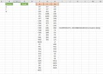
Hi I just got to my computer. Unfortunately I don't have the same capabilities on my smart phone. I sent an image which you ask for earlier. I described them as dept. and position earlier for I thought it may be less confusing. In the image you see there are more than the three. Actually there will be about around 6 and the ranks will vary in number of rows. I included something that I used for my punctuation in the other column you helped me out earlier. Thank you,

 

[sparky2205]

I'm afraid you have me really confused now.
A, F & N are the Services in column B.
These are repeated as headers in columns F, G & H.
Under each of these I presumed were the Rank? (column D).
But in an earlier post you said the Rank (Position) was unique to the Service (Dept) or at least that's how I interpreted it.
From the post above it appears that's not the case and there is crossover between Service and Rank.

 

[Livin404]

I'm afraid you have me really confused now.
A, F & N are the Services in column B.
These are repeated as headers in columns F, G & H.
Under each of these I presumed were the Rank? (column D).
But in an earlier post you said the Rank (Position) was unique to the Service (Dept) or at least that's how I interpreted it.
From the post above it appears that's not the case and there is crossover between Service and Rank.

They are not meant to be repeats or anything. They were to show what ranks go with the letters. The actual list what you saw is on a second worksheet which will be hidden. I put it like that so I wouldn’t have to make two screen shots. So the letter you see Have to have rank from the list and post it to the column.