louisli_evo
New Member
- Joined
- Mar 11, 2020
- Messages
- 11
- Office Version
- 365
- Platform
- Windows
Hi, I'm modifying an old worksheet to add an ability to check if some data throughout 12 months of a year has been correctly filled. I have verified the condition on separate cells but seems conditional formatting doesn't read the same formula syntax.
Sheet "Figures":

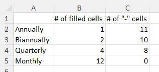
For example, if the frequency is "Annually", then it checks cells F2-Q2 if one of the cells is filled (or if eleven (11) hyphens "-" are left). If the frequency is quarterly, it checks cells F2-Q2 if four of the cells are filled (or if eight (8) hyphens "-" are left). If this condition is true, the background of "Frequency" changes to "no colour".
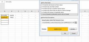
I applied conditional formatting on this "Frequency" column (D), with the formula:
The Frequency on this sheet is just a reference to another cell in the sheet "Figures".
And the Frequency on "Metrics" sheet has the following options (using data validation, from a list on sheet "(Controls)")
- Annually
- Biannually
- Quarterly
- Monthly
So, this is what I put on sheet "(Controls")

Did I miss anything? It seems close but I just couldn't figure out what's the problem.
Thank you very much.
Sheet "Figures":
For example, if the frequency is "Annually", then it checks cells F2-Q2 if one of the cells is filled (or if eleven (11) hyphens "-" are left). If the frequency is quarterly, it checks cells F2-Q2 if four of the cells are filled (or if eight (8) hyphens "-" are left). If this condition is true, the background of "Frequency" changes to "no colour".
I applied conditional formatting on this "Frequency" column (D), with the formula:
="COUNTIF(F2:Q2,"-")==VLOOKUP('Figures'!D2,'(Controls)'!A2:C5,3)"The Frequency on this sheet is just a reference to another cell in the sheet "Figures".
=Metrics!G2And the Frequency on "Metrics" sheet has the following options (using data validation, from a list on sheet "(Controls)")
- Annually
- Biannually
- Quarterly
- Monthly
So, this is what I put on sheet "(Controls")
Did I miss anything? It seems close but I just couldn't figure out what's the problem.
Thank you very much.